In the previous lesson, we studied the numerical solution of the linear and non-linear convection equations, using the finite-difference method. We began by discretizing the one-way wave equation using a classic forward-time/backward space scheme, and computing the solution using an initial condition consisting of a square pulse.
Computing with finer spatial grids while keeping the time step constant, you encountered four cases:
a coarse run with
nx=41smoothed the square pulse and attenuated its height,a finer run with
nx=81improved the solution, but smoothing still ocurred,a surprising case with
nx=101matched the exact solution, anda further refinement with
nx=121destroyed the solution.
In this lesson, we will explore why changing the discretization parameters can affect your solution in such a drastic way. The central question we want to answer is:
Why did refining the spatial grid improve the linear-convection calculation, make it an exact grid shift at one setting, and then destroy it?
Let’s begin by importing our favorite Python libraries for numerical computing.
import numpy as np
import matplotlib.pyplot as plt
# Set the font family and size to use for Matplotlib figures.
plt.rcParams['font.family'] = 'serif'
plt.rcParams['font.size'] = 12The code below corresponds to the same function we used in the previous lesson, but incorporating the vectorized update in space, leaving only the loop in time. Be sure to review the way array slicing works in this code, sketched in Figure 5 of Lesson 6, and the Python refresher that came after.
def advance_linear_convection(u0, c, dx, dt, num_steps):
    '''Advance linear convection with the FTBS scheme.'''
    u = u0.copy()
    for n in range(num_steps):
        u[1:] = u[1:] - c * dt / dx * (u[1:] - u[:-1])
    return u
How far does the wave travel in one step?
Look again at the discretized equation implemented by our function:
Pay attention to the coefficient multiplying the spatial difference: c * dt / dx. The speed has units of distance per time, so is the distance the exact wave travels during one time step. Dividing by the grid spacing expresses that distance in grid intervals. We give this dimensionless ratio a name:
This is the Courant number, also known as the CFL number (Courant–Friedrichs–Lewy) Courant et al., 19281967. For the positive speed considered here, means that the wave travels eight-tenths of a grid interval per time step; means one complete interval.
The ratio is already present in Equation 1 and in our code. Refining the spatial grid while keeping the time step fixed makes smaller and the Courant number larger. What values did it take in the four runs from the previous lesson?
On paper
Use , , and , as in Lesson 6. For each of nx = 41, 81, 101, 121, calculate and then . Check that the units cancel. Interpret each result as the distance traveled in one step, measured in grid intervals, and match it to the behavior you observed.
L = 2.0
c = 1.0
dt = 0.02
nx_trials = [41, 81, 101, 121]

print(f"{'nx':>5} {'dx':>10} {'C':>8}")
for nx in nx_trials:
    dx = L / (nx - 1)
    courant = c * dt / dx
    print(f'{nx:5d} {dx:10.5f} {courant:8.3f}')
The four Courant numbers are 0.4, 0.8, 1.0, and 1.2. The run that shifted the pulse exactly had ; the failed run had . These observations suggest that this ratio matters, but they do not yet explain the failure or establish a stability condition.
To investigate, we will ask a more focused question: what happens to a small disturbance in the initial data?
Perturbation study
In your notebook
Reconstruct this experiment in your own notebook, using the vectorized advance_linear_convection() function above. Before running it, predict how a disturbance of 10-3 will behave on each of the three grids. Build the paired initial states and record their maximum difference after every step. You may copy the plot formatting and table layout. Compare your results with your predictions, and explain what the experiment does and does not establish about stability.
Imagine running the same calculation twice, with just one initial value changed by 10-3 in the second run. Both runs use the same grid, time step, method, and inflow value. Does their difference remain small as we advance in time, or does the calculation amplify it?
Use a constant background, , so that the disturbance is easy to isolate. In the second array, add 10-3 at . The unperturbed exact solution stays constant; the equation transports a disturbance without increasing its height. Our numerical update may behave differently.
We will repeat this paired experiment on nx = 81, 101, 121, keeping and . These are the three runs with , 1.0, and 1.2. Advance each pair for 25 steps, reaching the same physical time on every grid.
At each step, measure the largest absolute difference between the two arrays:
Here, denotes the unperturbed run and the perturbed run. Initially, . Taking absolute values matters because a disturbance can develop both positive and negative differences.
The perturbation occupies one grid point, so its physical width changes with the grid. We are testing how the method amplifies a grid disturbance; this is not a convergence comparison for one fixed continuous initial profile.
num_steps = 25
perturbation = 1e-3
nx_perturbation = [81, 101, 121]
time = dt * np.arange(num_steps + 1)
error_histories = []
courant_numbers = []
Each run starts from fresh arrays. The point at nx // 4 lies at on all three grids; // is integer division. The left boundary remains in both runs, because the function updates only u[1:].
We call advance_linear_convection() with num_steps=1 to inspect the difference after every step. This uses the same update as advancing all 25 steps at once, while letting us record its behavior along the way. The FTBS stencil can pass a disturbance at most one grid point to the right per step. Even on the coarsest grid, the perturbed point is more than 25 grid intervals from the outflow, so the disturbance cannot leave the array during this experiment.
Before running: predict which of the three cases will reduce, preserve, or amplify the maximum difference. Treat the prediction as a hypothesis to test.
for nx in nx_perturbation:
    dx = L / (nx - 1)
    courant = c * dt / dx

    u_a = np.ones(nx)
    u_b = u_a.copy()
    u_b[nx // 4] += perturbation

    error = np.empty(num_steps + 1)
    error[0] = np.max(np.abs(u_b - u_a))
    for n in range(num_steps):
        u_a = advance_linear_convection(u_a, c, dx, dt, 1)
        u_b = advance_linear_convection(u_b, c, dx, dt, 1)
        error[n + 1] = np.max(np.abs(u_b - u_a))

    error_histories.append(error)
    courant_numbers.append(courant)
Let’s plot the recorded differences. A logarithmic vertical scale lets us see shrinking and growing disturbances on the same axes. Equal vertical distances represent equal multiplicative changes, rather than equal additive changes.
fig, ax = plt.subplots(figsize=(6.0, 3.5))
for courant, error in zip(courant_numbers, error_histories):
    ax.semilogy(time, error, label=f'C = {courant:.2f}')

ax.axhline(perturbation, color='black', linestyle=':',
           label='Initial disturbance')
ax.set_xlabel('Time')
ax.set_ylabel('Maximum difference between runs')
ax.grid(which='both', alpha=0.3)
ax.legend()
fig.tight_layout();
A few selected steps make the amount of amplification easier to compare:
steps_to_report = [1, 5, 10, 25]
print(f"{'C':>6}" + ''.join(
    f'{str(step) + " steps":>14}' for step in steps_to_report
))
for courant, error in zip(courant_numbers, error_histories):
    print(f'{courant:6.2f}' + ''.join(
        f'{error[step]:14.2e}' for step in steps_to_report
    ))
For , the maximum difference decreases as the disturbance spreads over neighboring points. For , its maximum stays at 10-3. For , a difference initially one-thousandth of the background grows to about 1 after only 25 steps. The calculation has turned a small change in the initial data into a large change in the result.
This is the question behind numerical stability: does the method control the amplification of small disturbances? More precisely, over a fixed physical time interval, we seek a bound on amplification that remains independent of the mesh as we refine it under the stated conditions. Stability need not mean that every disturbance decays; the result illustrates controlled propagation without decay.
These three runs provide evidence for particular choices of grid and time step. They do not prove a general bound. We still need to explain why the coefficient in Equation 1 separates these behaviors.
Self-checks
For each Courant number, divide the final maximum difference by the initial maximum difference. What amplification factor do you obtain over ?
Why would running only the constant, unperturbed state fail to expose the growing disturbance?
Does the decreasing difference at establish that this grid gives an accurate transported pulse? Relate your answer to the smoothing observed in Lesson 6.
Where does the information come from?
We introduced the Courant number by asking how far the exact wave travels during one time step. Now turn that question around: where was the information needed at one time step earlier?
For constant positive speed , the solution travels along a characteristic without changing its value. Tracing that characteristic backward from gives
The exact solution therefore needs the value at . Our numerical update, Equation 1, uses only two old values: and . Figure 1 puts these two descriptions on the same space–time diagram.
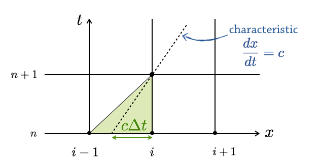
Figure 1:The FTBS update uses the two black points at time level . The dashed characteristic traces the exact solution back a distance . The shaded triangle connects the numerical inputs to the new point; the illustrated characteristic lands between them.
In the case drawn, : the characteristic lands between and . At , it lands exactly on . For , it lands farther to the left, outside the interval spanned by the two input points.
This is the local picture of a domain of dependence: the earlier data that can influence a particular solution value. To see its meaning over several steps, trace the stencil backward again. Two steps earlier, the FTBS value can depend on points , , and ; after steps, its numerical dependence extends at most from to . The exact characteristic reaches over the same interval. We are considering points whose backward stencils remain inside the spatial domain; at an inflow boundary, the prescribed boundary data also enter the dependence.
For the characteristic to stay within the numerical dependence interval, we need
We have assumed positive speed and positive step sizes. The limiting case corresponds to no travel during a step. Notice that equality is allowed: traveling exactly one grid interval does not put the required information beyond the stencil.
If , the exact wave travels farther during a fixed time interval than information can pass through the numerical stencil. Refining with that same supercritical Courant number does not remove the mismatch. The numerical method cannot, in general, converge to a solution that depends on data it cannot reach. This information-containment requirement is the CFL condition for the stencil considered here.
On paper
Sketch the backward characteristic for , 1.0, and 1.2, starting from the same new grid point. Mark the two old grid points used by FTBS. Where does each characteristic land? Then trace two numerical steps backward and identify the three old points that can influence the new value.
The geometry explains why is a meaningful threshold, but it does not tell us how the update combines the available values. Containing the characteristic is a necessary condition for convergence of these explicit transport schemes; it is not, by itself, a proof that disturbances remain controlled. To explain the decay, preservation, and growth measured in our perturbation study, we will next examine the weights multiplying the two old values.
How the update controls a disturbance
We can establish a stability bound directly from the update. First, collect the terms multiplying each old value in Equation 1:
When , the two weights, and , are nonnegative and sum to one. The new value is therefore a weighted average of the two old values: it lies between them. Such an average is called a convex combination.
To explain the perturbation experiment, we need to apply this observation to the difference between the two runs.
Subtract the two updates
Let and denote the unperturbed and perturbed runs, and write their difference as
Here, is the difference between two numerical solutions, not the error relative to an exact solution. Both runs use the same , , and , so their updates have the same weights:
Subtract the first update from the second and collect the differences:
The difference obeys the same update as the solution. This follows from the linearity of this scheme with constant speed; we cannot assume it for a nonlinear update.
Bound the largest difference
The quantity measured in our experiment was
Every old difference has magnitude at most . To bound the new difference, use the triangle inequality: the magnitude of a sum is no larger than the sum of the magnitudes. For , the weights are nonnegative, giving
This bounds every updated point, including the rightmost point. At the left boundary, both runs keep the same prescribed value, so their difference is zero. Taking the maximum over the whole array therefore gives . Repeating the argument over successive steps yields
The largest initial disturbance cannot be amplified. This bound holds for any initial difference, not just the single-point disturbance we tested. Its amplification bound is one, independent of the grid spacing and number of steps: it establishes stability for the stated scheme and boundary treatment.
Read the experiment again
The decrease observed at is consistent with Equation 12. The bound permits this decrease, but does not require every disturbance to decay.
At , Equation 9 becomes : the disturbance shifts one grid point to the right at each step. Its maximum stays unchanged while it remains in the domain, exactly as we measured. The same shift explains the square-pulse result from Lesson 6. Equality belongs in the stability condition.
At , the weight is negative, so the nonnegative-weight argument no longer applies. That alone does not prove growth. Our experiment has exhibited a growing disturbance; an analytical explanation of that growth is the next question.
On paper
Starting from the two numerical updates, reconstruct the argument without looking at the worked derivation:
Subtract the updates to obtain an equation for .
Use the triangle inequality and to show that . Identify exactly where you need .
Explain why identical inflow values matter when taking the maximum over the whole array.
State what the bound tells you about the experiment at and , and why it does not explain the growth at .
A disturbance that grows when 
To prove that the method can amplify a disturbance, we only need to find one that grows. Choose a perturbation whose sign alternates at neighboring grid points:
For even , ; for odd , . The initial differences therefore look like , all with magnitude . We can make as small as we like.
This is a different disturbance from the single-point perturbation in our experiment. We choose it because adjacent differences are exact opposites, which makes its evolution easy to calculate. For now, consider an alternating pattern extending over the grid without boundaries; we will return to the finite interval below.
Follow one update
Suppose the difference at step has the form
where is its signed amplitude and . Its left neighbor has the opposite sign:
Substitute both expressions into Equation 9:
The alternating pattern is preserved. Only its amplitude changes, according to
We call the amplification factor for this pattern. Its sign tells us whether the signs flip at each step; its magnitude tells us whether the disturbance shrinks, stays the same size, or grows.
Repeat the update
Starting from , successive steps give
Continuing in the same way,
Now let . Then , so
The magnitude increases at every step, and the signs reverse. For example, at , : each step multiplies the magnitude by 1.4. After 20 steps, it is about 837 times its initial value. Even an arbitrarily small initial disturbance can be amplified by a large factor.
At , : the signs flip but the magnitude stays unchanged, consistent with shifting an alternating pattern by one grid point. At , , so its magnitude decreases by a factor of 0.6 per step. These factors describe this alternating pattern; they do not give the maximum difference for the earlier single-point disturbance.
What about the boundary and a fixed final time?
Our numerical runs have a prescribed left boundary, with zero difference between the two inflow values. We cannot impose the alternating pattern at that boundary as well. Instead, set and alternate the initial differences at the interior points.
After steps, the backward stencil of point reaches only as far as . Thus, at points more than grid intervals from the left boundary (), all the initial differences contributing to the update belong to the alternating pattern. Equation 19 holds there exactly. A numerical check of this prediction must use such points, rather than a region already influenced by the inflow.
To connect growth to our definition of stability, hold and a physical final time fixed. With ,
using grids for which is an integer number of steps. As decreases, increases. The amplification therefore grows without bound. On our finite domain, choose a sufficiently short fixed so that an interior point satisfies throughout refinement. The growing pattern at that point then remains unaffected by the inflow. Since the maximum difference is at least as large as the difference at that point, there can be no mesh-independent amplification bound.
Together, the two arguments establish the sharp condition for this FTBS scheme with the boundary treatment considered: within that interval, no initial difference is amplified in maximum magnitude; for , an alternating initial difference provides a counterexample. This does not mean every initial state grows when —a constant state, for example, remains constant. Stability must control all admissible small disturbances.
On paper
Starting from neighboring differences and , calculate one update at . Check its sign and magnitude against .
Predict the alternating disturbance’s magnitude after 20 steps at , 1.0, and 1.2, as a multiple of its initial magnitude.
Explain why a finite-grid check after 20 steps should sample points more than 20 grid intervals from the left boundary.
Make a robust solver with an agent
Our short function makes FTBS easy to inspect, but it leaves its assumptions to the user (a.k.a. caller). We now know enough to build a solver that enforces those assumptions, chooses a stable time step, and reaches a requested final time. An agent can draft the validation and tests while the numerical reasoning is fresh in our minds.
The activity below supplies the design. Your job is to turn it into a clear specification, inspect the agent’s implementation, and establish whether its tests provide useful evidence. The result will solve constant-speed transport on a uniform grid with constant inflow; it will not decide whether that model or grid is appropriate for an engineering application.
With an Agent
Turn the understood upwind algorithm into a reusable solver with input checks and automatic time-step selection. You will organize the supplied requirements into a specification, ask an agent to draft the solver and tests, and audit both against independent expectations. A deliberately incorrect boundary value will check whether the tests detect a meaningful defect. Your final verdict will state what the improved solver guarantees and what remains your responsibility.
1. Diagnose four weaknesses
The following calls all return arrays without raising an exception. Use a small initial profile so that you can inspect the results directly. Its grid is , so the spacing is 1.
u_demo = np.array([1.0, 2.0, 1.0, 1.0])

# A step beyond the stability bound.
print('C > 1:       ', advance_linear_convection(
    u_demo, c=1.0, dx=1.0, dt=1.2, num_steps=1))

# A negative speed with the same backward-space update.
print('Negative c:  ', advance_linear_convection(
    u_demo, c=-1.0, dx=1.0, dt=0.2, num_steps=1))

# Integer storage for a calculation with fractional updates.
print('Integer u0:  ', advance_linear_convection(
    u_demo.astype(int), c=1.0, dx=1.0, dt=0.2, num_steps=1))

# A spacing inconsistent with the grid on which u_demo was defined.
print('Wrong dx:    ', advance_linear_convection(
    u_demo, c=1.0, dx=2.0, dt=0.2, num_steps=1))
With the intended positive-speed update at , the result would be [1.0, 1.8, 1.2, 1.0]. Compare that reference with the outputs and use the table to explain each weakness.
| Weakness | Mechanism | Design response |
|---|---|---|
| An unsupported step can create overshoots and amplify disturbances. | Choose the time step from a valid target Courant number. | |
| Negative speed | Backward differencing uses the wrong direction, even when $ | C |
Integer u0 | Assignment into an integer array discards fractional parts. | Make a floating-point working copy. |
Incorrect dx | The function cannot check spacing against a grid it never receives. | Construct a uniform grid from domain limits and the length of u0. |
A visible failure can still justify a check before computation. For the last case, another conditional in the old function cannot recover missing information: we need a better interface.
In your notebook
Keep the original solver as a reference. Reproduce the four calls and explain each result using the update, including the fractional values lost in the integer case. Then follow the derivations and complete the supplied specification template before contacting an agent. You may copy the interface, requirement tables, and mechanical formatting.
2. Derive the numerical requirements
For , information arrives from the right. Replace the backward difference with a forward difference:
Here is signed. The weights and are nonnegative and sum to one when . Together with the positive-speed result, this gives , provided the spatial difference uses the upstream neighbor. Hold the left endpoint fixed for and the right endpoint fixed for . Because the speed is constant, choose the direction once per solver call. For , the state does not change.
Next, let be a target Courant magnitude, with . For nonzero speed and requested duration , choose
The ceiling rounds up to an integer number of steps. Consequently , while in exact arithmetic. Report the realized signed , whose magnitude may be smaller than . Handle or separately, before any division that assumes nonzero values.
On paper
Derive the two weights in Equation 22 and their allowed interval. Calculate one step from
[1, 2, 3, 4]with , keeping the right inflow fixed.For , , , and , calculate the step limit, , the actual step, and the realized Courant number. Explain why rounding down would violate the target.
3. Use this design brief
The new interface is
solve_transport(u0, x_limits, c, t_final, courant=0.8, max_steps=100_000)u0 represents values at equally spaced points including both domain endpoints. The solver constructs x from x_limits and len(u0), and derives dx. It cannot check whether the caller actually sampled the intended profile at those locations.
For this exercise, assume ordinary real numeric lists, NumPy arrays, and scalar parameters, with magnitudes for which grid and time-step calculations are representable in floating point. We do not require general-purpose type validation or special handling of extreme floating-point ranges. courant is the target magnitude , not the signed realized .
| Requirement | Required behavior |
|---|---|
| Initial state | Make a floating-point copy. Check that it is one-dimensional and contains at least two finite values. |
| Domain | Check that x_limits contains two finite limits with x_min < x_max. Construct an endpoint-inclusive uniform grid and derive its spacing. |
| Parameters | Check that speed, final time, and target Courant number are finite; require t_final >= 0 and 0 < courant <= 1. Check that max_steps is a positive integer. |
| Time and budget | For nonzero speed and duration, use Equation 23. Reject a step count above max_steps before advancing. Do not shorten the requested duration. |
| Evolution | Use vectorized upwind differences with old-time-level values. Hold the initial left endpoint for positive speed and the initial right endpoint for negative speed; update through the downstream endpoint. |
| No evolution | After the input checks, return an unchanged floating-point copy for zero speed or zero duration, with zero steps, dt=0, and realized courant=0. For zero speed, the solution is unchanged at the requested final time. |
| Ownership | Do not modify the input arrays or share their storage with returned arrays. |
| Refused requests | Raise ValueError with a message identifying a failed check or an exceeded step budget. Do not return a partial result. |
Return a dictionary with these keys:
| Key | Meaning |
|---|---|
x, u | Constructed grid and final solution as floating-point arrays |
t_final | Requested time reached, up to floating-point arithmetic |
dx, dt | Grid spacing and actual time step |
num_steps | Number of completed updates |
courant | Realized signed Courant number |
The step budget is a simple limit on requested work, not a runtime or memory guarantee. Nonuniform grids, variable speeds, and changing inflow values are outside this solver’s scope. Keep the implementation focused on this brief.
4. Put the brief into a specification
Copy the template below into your notebook and fill it from the brief. You are organizing supplied requirements, not inventing a new solver design. For each validation requirement, name the defect or assumption it addresses and one way to check the promised behavior.
Outcome: What calculation should this solver deliver?
Context and assumptions: What equation, grid, and boundary model does it support?
Interface and outputs: Copy the signature and define every returned field.
Required behavior: State the update, direction selection, time selection,
    copying rules, and zero-evolution cases.
Rejected requests: List invalid inputs and the required exception behavior.
Acceptance evidence: Map each requirement to a hand result, invariant,
    comparison, or rejected-call test.
Agent permissions: State what the agent may add and what it must preserve.
Use the independent expectations in subsection 6 to complete the evidence section. If a requirement is unclear to you, resolve it against the brief before asking the agent to implement it.
5. Ask an agent to implement and test it
Attach your working notebook, including the original solver, derivations, and completed specification. Use this prompt:
Implement solve_transport according to the specification in my notebook.
Use the displayed FTBS update for positive speed, the derived forward-space
update for negative speed, and the derived final-time step selection.

Add only new, unexecuted cells at the end: one implementation cell, one
cell containing tests, and one short markdown cell mapping the tests to
requirements and identifying any limitations. Use only NumPy and the Python
standard library. Keep the numerical updates visible in the function and
use triple-single-quoted docstrings. Do not add a package or testing framework.

Use straightforward checks for the stated contract. Do not broaden the
accepted input types or add general-purpose validation machinery. Assume
ordinary real numeric inputs in representable ranges, as stated in the brief.
Do not add special handling for mixed Boolean data, extreme floating-point
values, or roundoff-triggered changes to the step count. Identify concerns
outside the contract in a short limitations note rather than implementing them.

Preserve every existing cell. Do not execute code, install anything, access
external resources, or write my verdict. If the specification has a
consequential ambiguity, ask rather than invent behavior.

Write callable tests using assertions and numpy.testing. Give them a
run_solver_checks(solver) entry point so I can test a deliberately defective
replacement later. Use the independent expected values in my specification;
do not compute expected answers by duplicating the solver's algorithm.
Use the supplied acceptance cases to test the checks, reported quantities,
and numerical results, including both speed directions. Keep the suite small. For refused calls, check the exception type and that
the message explains the failed requirement, without requiring exact wording.
The agent supplies implementation and test-writing labor. You remain responsible for checking both: a passing test written from the same mistaken assumption as the solver is weak evidence.
6. Audit, run, and defend the result
Before executing, inspect the function against your specification. Check that conversion to floating point precedes evolution, the two slices use old values, negative speed changes both stencil and inflow endpoint, and the time-selection and budget checks occur before the loop. Inspect the tests too: do they use independent answers and actually exercise the intended branch?
Use these acceptance cases. Unless stated otherwise, use floating-point inputs and the default step budget.
| Case | Inputs or action | Independent expectation |
|---|---|---|
| One positive step | u0=[1,2,3,4], limits (0,3), c=1, T=0.2, target 0.2 | u=[1,1.8,2.8,3.8]; one step |
| One negative step | Same, but c=-1 | u=[1.2,2.2,3.2,4]; right endpoint preserved |
| Exact shifts | Same initial data and limits, T=1, target 1, speeds 1 and -1 | Respectively [1,1,2,3] and [2,3,4,4] |
| Final-time selection | Five points on (0,1), c=1, T=0.55, target 0.8 | dx=0.25, three steps, dt=0.55/3, realized ; N*dt agrees with T |
| Constant state | [2,2,2,2], both speed directions | All values remain 2 |
| Integer input | Repeat a fractional-step case with integer and floating arrays | Same floating-point result, including fractional values |
| Ownership | Save input copies, solve, then modify the returned arrays | Input values remain unchanged |
| Zero evolution | Valid inputs with zero speed or zero duration | Unchanged floating-point copy and the specified zero-step metadata |
| Invalid requests | Try one-point, two-dimensional, and nonfinite states; reversed limits; negative duration; nonfinite speed; targets 0 and 1.2; a zero step budget | Each raises ValueError identifying the failed check |
| Exceeded budget | The three-step final-time case above with max_steps=2 | Raises before evolution; does not return a shortened run |
Use np.testing.assert_allclose for computed floating-point values; small roundoff differences are not implementation defects. Use exact checks for step counts, required keys, and exception types. In the final-time case, allow a small floating-point tolerance when checking that the realized Courant magnitude does not exceed the target; this is a comparison tolerance, not permission to choose a materially larger step.
After reviewing the cells, run the tests yourself. Record each failure as an implementation defect, a faulty test, or a specification ambiguity, with a reason. Send the agent a focused revision request and rerun affected checks after inspecting the change.
Finally, check that the tests can detect a known mistake. Add this temporary replacement in your working notebook; it deliberately corrupts the right inflow for negative speed when endpoint values differ:
def solve_transport_wrong_inflow(u0, x_limits, c, t_final,
                                 courant=0.8, max_steps=100_000):
    '''Deliberately impose the wrong inflow value for negative speed.'''
    result = solve_transport(u0, x_limits, c, t_final,
                             courant=courant, max_steps=max_steps)
    if c < 0 and result['num_steps'] > 0:
        result['u'][-1] = float(u0[0])
    return result

run_solver_checks(solve_transport_wrong_inflow)
An assertion should fail on a negative-speed case with unequal endpoint values. Identify that test and explain the mismatch. If the suite passes, it has missed the injected defect: improve the test, not the defective replacement. Keep this deliberate failure separate from the cell that runs the checks on the accepted solver.
Your verdict
State whether you accept the solver, and support your decision with the executed checks and defect-injection result. Identify a change you required, or explain why the first draft met the brief. Name the assumptions now enforced, the automatic choices reported to the caller, and what the tests still do not establish. In particular, stable evolution does not certify the physical model or sufficient spatial accuracy. Include a short agent record with the specification, prompts, accepted or revised work, and verification you performed.
Debrief: what became more robust?
The caller no longer has to coordinate grid spacing, time step, spatial bias, inflow endpoint, and step count by hand. The solver handles those dependent choices, reports what it did, and refuses the invalid requests named in its contract. The tests provide evidence that the promised behavior is implemented, and the injected defect checks that an important test can fail for the right reason.
These are real responsibilities in scientific software. We collected them in one small function so that you could inspect them. In a larger application, input processing, mesh and field objects, solver routines, and a separate test suite can share these responsibilities. A numerical update need not repeat every input check at every step. Where to put a check, and what it costs, are design decisions.
This solver has a deliberately limited contract. We have not investigated every input type, overflow or underflow, or extreme grid and time scales. Nor do passing tests and a stable update establish convergence, sufficient accuracy on the chosen grid, or a valid physical model. Further use requires evidence appropriate to that use; high-consequence work would demand much more than this notebook exercise.
The agent reduces the labor of drafting implementation and tests. It does not remove the work of understanding the contract, inspecting the code, and obtaining independent evidence. Judge the improvement by the failures prevented and the behavior verified, rather than by the number of checks the agent adds.
- Courant, R., Friedrichs, K., & Lewy, H. (1928). Über die partiellen Differenzengleichungen der mathematischen Physik. Mathematische Annalen, 100(1), 32–74. 10.1007/BF01448839
- Courant, R., Friedrichs, K., & Lewy, H. (1967). On the partial difference equations of mathematical physics. IBM Journal of Research and Development, 11(2), 215–234. 10.1147/rd.112.0215