In the first module, we studied numerical integration methods for the solution of ordinary differential equations (ODEs), using the phugoid model of glider flight as a motivation. In this module, we will study the numerical solution of partial differential equations (PDEs), where the unknown is a multi-variate function. The problem could depend on time, , and one spatial dimension (or more), which means we need to build a discretization grid with each independent variable.
We will start our discussion of numerical PDEs with 1D linear and non-linear convection equations, the 1D diffusion equation, and 1D Burgers’ equation.
1D linear convection
The one-dimensional linear convection equation is the simplest, most basic model that can be used to learn something about numerical solution of PDEs. It’s surprising that this little equation can teach us so much! Here it is:
The equation represents a wave propagating with speed in the direction, without change of shape. For that reason, it’s sometimes called the one-way wave equation (sometimes also the advection equation).
With an initial condition , the equation has an exact solution given by:
Go on: check it. Take the time and space derivative and stick them into the equation to see that it holds.
Look at the exact solution for a moment ... we know two things about it:
its shape does not change, being always the same as the initial wave, , only shifted in the -direction; and
it’s constant along so-called characteristic curves, constant. This means that for any point in space and time, you can move back along the characteristic curve to to know the value of the solution.
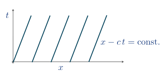
Figure 1:Characteristic curves for a positive convection speed .
Why do we call the equations linear? PDEs can be either linear or non-linear. In a linear equation, the unknown function and its derivatives appear only in linear terms, in other words, there are no products, powers, or transcendental functions applied on them.
The most important feature of linear equations is: solutions can be superposed to generate new solutions that still satisfy the original equation. This is super useful!
Finite-differences
In the previous lessons, we discretized time derivatives; now we have derivatives in both space and time, so we need to discretize with respect to both these variables.
Imagine a space-time plot, where the coordinates in the vertical direction represent advancing in time—for example, from to —and the coordinates in the horizontal direction move in space: consecutive points are , , and . This creates a grid where a point has both a temporal and spatial index. Here is a graphical representation of the space-time grid:
For the numerical solution of , we’ll use subscripts to denote the spatial position, like , and superscripts to denote the temporal instant, like . We would then label the solution at the top-middle point in the grid above as follows: .
Each grid point below has an subscript index, corresponding to the spatial position and increasing to the right, and an superscript index, corresponding to the time instant and increasing upwards. A small grid segment would have the following values of the numerical solution at each point:
Another way to explain our discretization grid is to say that it is built with constant steps in time and space, and , as follows:
Discretizing our model equation
Let’s see how to discretize the 1D linear convection equation in both space and time. By definition, the partial derivative with respect to time differentiates only with time and not with space; its discretized form changes only the indices. Similarly, the partial derivative with respect to differentiates with space not time, and only the indices are affected.
We’ll discretize the spatial coordinate into points indexed from to , and then step in discrete time intervals of size .
From the definition of a derivative (and simply removing the limit), we know that for sufficiently small:
This formula could be applied at any point . But note that it’s not the only way that we can estimate the derivative. The geometrical interpretation of the first derivative at any point is that it represents the slope of the tangent to the curve . In the sketch below, we show a slope line at and mark it as “exact.” If the formula written above is applied at , it approximates the derivative using the next spatial grid point: it is then called a forward difference formula.
But as shown in the sketch below, we could also estimate the spatial derivative using the point behind , in which case it is called a backward difference. We could even use the two points on each side of , and obtain what’s called a central difference (but in that case the denominator would be ).
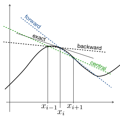
Figure 2:Forward, backward, and central finite-difference approximations to the slope at .
We have three possible ways to represent a discrete form of :
Forward difference: uses and ,
Backward difference: uses and ,
Central difference: uses two points on either side of .
The sketch above also suggests that some finite-difference formulas might be better than others: it looks like the central difference approximation is closer to the slope of the “exact” derivative. We’ll see later how to make this observation rigorous.
The three formulas are:
Euler’s method is equivalent to using a forward-difference scheme for the time derivative. Let’s stick with that, and choose the backward-difference scheme for the space derivative. Our discrete equation is then:
where and are two consecutive steps in time, while and are two neighboring points of the discretized coordinate. With given initial conditions, the only unknown in this discretization is . We solve for this unknown to get an equation that lets us step in time, as follows:
It is useful to sketch a grid segment, showing the grid points that influence our numerical solution. This is called a stencil. Below is the stencil for solving our model equation with the finite-difference formula we wrote above.
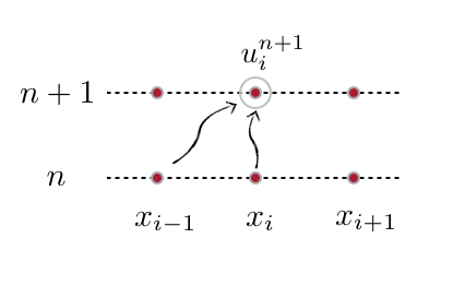
Figure 3:Stencil for the forward-time, backward-space discretization of linear convection.
And compute!
Alright. Let’s get a little Python on the road. First: we need to load our array and plotting libraries, as usual.
In your notebook
Create a new, clean notebook for your work rather than executing the code cells in this lesson from top to bottom. Keep the lesson open as a reference and reconstruct the calculation there.
Type the grid definition, square-wave initial condition, FTBS update, and time loop yourself so that you can trace the numerical update back to Equation 9. Before running each experiment, record what you expect the wave to do. Reproduce the fixed-dt grid experiment and the controlled refinement study later in the lesson; compare the controlled study with the order you derive on paper. In the nonlinear section, implement and check both updates yourself before delegating the comparison to an agent. You may copy mechanical details such as imports and plot formatting when transcription would add no understanding.
Consult Reconstruct a lesson for the general workflow.
import numpy as np
import matplotlib.pyplot as plt
We also set notebook-wide plotting parameters for the font family and the font size by modifying entries of the rcParams dictionary.
# Set the font family and size to use for Matplotlib figures.
plt.rcParams['font.family'] = 'serif'
plt.rcParams['font.size'] = 10
As a first exercise, we’ll solve the 1D linear convection equation with a square wave initial condition, defined as follows:
We also need a boundary condition on : let at . Our spatial domain for the numerical solution will only cover the range .
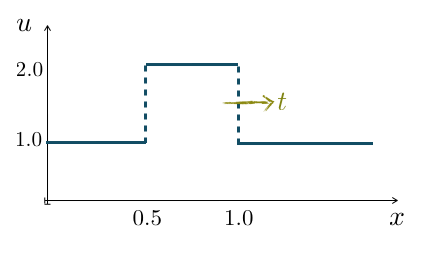
Figure 4:Square-wave initial condition with a unit background and a pulse of height 2.
Now let’s define a few variables; we want to make an evenly spaced grid of points within our spatial domain. In the code below, we define a variable called nx that will be the number of spatial grid points, and a variable dx that will be the distance between any pair of adjacent grid points. We also can define a step in time, dt, a number of steps, nt, and a value for the wave speed: we like to keep things simple and make .
# Set parameters.
nx = 41    # number of spatial discrete points
L = 2.0    # length of the 1D domain
dx = L / (nx - 1)  # spatial grid size
nt = 25    # number of time steps
dt = 0.02  # time-step size
c = 1.0    # convection speed

# Define the grid point coordinates.
x = np.linspace(0.0, L, num=nx)
We also need to set up our initial conditions. Here, we use the NumPy function np.ones() defining an array which is nx-element long with every value equal to 1. How useful! We then change a slice of that array to the value , to get the square wave, and we print out the initial array just to admire it. But which values should we change? The problem states that we need to change the indices of u such that the square wave begins at and ends at .
We can use the np.where() function to return a list of indices where the vector meets some conditions.
The function np.logical_and() computes the truth value of x >= 0.5 and x <= 1.0, element-wise.
# Set initial conditions with 1.0 everywhere (for now).
u0 = np.ones(nx)
# Get a list of indices where 0.5 <= x <= 1.0.
mask = np.where(np.logical_and(x >= 0.5, x <= 1.0))
print(mask)
With the list of indices, we can now update our initial conditions to get a square-wave shape.
# Set initial condition u = 2.0 where 0.5 <= x <= 1.0.
u0[mask] = 2.0
print(u0)
Now let’s take a look at those initial conditions we’ve built with a handy plot.
# Plot the initial conditions.
plt.figure(figsize=(3.0, 3.0))
plt.title('Initial conditions')
plt.xlabel('x')
plt.ylabel('u')
plt.grid()
plt.plot(x, u0, color='tab:blue', linestyle='--', linewidth=2)
plt.xlim(0.0, L)
plt.ylim(0.0, 2.5);
It does look pretty close to what we expected. But it looks like the sides of the square wave are not perfectly vertical. Is that right? Think for a bit.
Now it’s time to write some code for the discrete form of the convection equation using our chosen finite-difference scheme.
For every element of our array u, we need to perform the operation:
We’ll store the result in a new (temporary) array un, which will be the solution for the next time-step. We will repeat this operation for as many time-steps as we specify and then we can see how far the wave has traveled.
We first initialize the placeholder array u to hold the values we calculate for the time step, beginning with a copy of the initial condition.
Then, we may think we have two iterative operations: one in space and one in time (we’ll learn differently later), so we may start by nesting a spatial loop inside the time loop, as shown below. You see that the code for the finite-difference scheme is a direct expression of the discrete equation.
Here, nt counts updates rather than stored time levels. Because range(nt) starts at zero and performs exactly nt passes, the final physical time in this example is nt * dt.
u = u0.copy()
for n in range(nt):
    un = u.copy()
    for i in range(1, nx):
        u[i] = un[i] - c * dt / dx * (un[i] - un[i - 1])
Note 1—We stressed above that our physical problem needs a boundary condition at . Here we do not need to impose it at every iteration because our discretization does not change the value of u[0]: it remains equal to one and our boundary condition is therefore satisfied during the whole computation!
Note 2—We will learn later that the code as written above is quite inefficient, and there are better ways to write this, Python-style. But let’s carry on.
Now compare the computed profile with the exact square wave translated to the same physical time.
# Evaluate the exact translated square wave at the final time.
t_final = nt * dt
u_exact = np.ones_like(x)
exact_mask = np.where(
    np.logical_and(x >= 0.5 + c * t_final,
                   x <= 1.0 + c * t_final)
)
u_exact[exact_mask] = 2.0

# Plot the numerical and exact solutions with the initial condition.
plt.figure(figsize=(3.0, 3.0))
plt.xlabel('x')
plt.ylabel('u')
plt.grid()
plt.plot(x, u0, label='Initial',
            color='tab:blue', linestyle='--', linewidth=1)
plt.plot(x, u_exact, label=f'Exact, t = {t_final:.2f}',
            color='tab:gray', linestyle='--', linewidth=2)
plt.plot(x, u, label=f'FTBS, t = {t_final:.2f}',
            color='tab:red', linestyle='-', linewidth=2)
plt.legend()
plt.xlim(0.0, L)
plt.ylim(0.0, 2.5);
That’s funny. Our square wave has definitely moved to the right, but it’s no longer in the shape of a top-hat. What’s going on?
Does a finer grid always help?
The rounded profile suggests that a finer spatial grid might improve the solution. Test that idea while keeping dt, nt, and fixed: only the number of spatial points changes below. Before executing the cell, predict what each refinement will do. Then compare the computed profiles with the exact translated square wave and record whether the numerical values remain between 1 and 2.
Treat this as an observation rather than a convergence study, and do not change dt to repair any surprising result. We will return to what happens—and why—in the next lesson.
# Change only the number of spatial points.
nx_trials = [41, 81, 101, 121]
fig, axes = plt.subplots(2, 2, figsize=(7.0, 7.0), sharex=True)

for ax, nx_trial in zip(axes.flat, nx_trials):
    dx_trial = L / (nx_trial - 1)
    x_trial = np.linspace(0.0, L, num=nx_trial)
    u_trial = np.ones(nx_trial)
    pulse = np.where(
        np.logical_and(x_trial >= 0.5, x_trial <= 1.0)
    )
    u_trial[pulse] = 2.0

    for n in range(nt):
        un_trial = u_trial.copy()
        for i in range(1, nx_trial):
            u_trial[i] = (
                un_trial[i]
                - c * dt / dx_trial
                * (un_trial[i] - un_trial[i - 1])
            )

    exact_trial = np.ones(nx_trial)
    exact_pulse = np.where(
        np.logical_and(
            x_trial >= 0.5 + c * t_final,
            x_trial <= 1.0 + c * t_final,
        )
    )
    exact_trial[exact_pulse] = 2.0

    ax.plot(x_trial, exact_trial, color='black',
            linestyle=':', linewidth=2, label='Exact')
    ax.plot(x_trial, u_trial, color='tab:red',
            linewidth=2, label='FTBS')
    ax.set_title(f'nx = {nx_trial}')
    ax.set_xlabel('x')
    ax.set_ylabel('u')
    ax.set_xlim(0.0, L)
    ax.grid()
    print(f'nx = {nx_trial:3d}: '          f'min(u) = {u_trial.min():8.3f}, '          f'max(u) = {u_trial.max():8.3f}')

axes.flat[0].legend()
fig.tight_layout();
Spatial truncation error
Recall the backward-difference approximation we are using for the spatial derivative:
We obtain it by using the definition of the derivative at a point, and simply removing the limit, in the assumption that is very small. But we already learned with Euler’s method that this introduces an error, called the truncation error.
We can determine the spatial order of this error by expanding in a Taylor series about . Complete that step on paper before reading the result.
On paper — derive the spatial truncation error
Derive the accuracy of the backward-difference formula independently of the computation:
Write the Taylor expansion of about , retaining terms through the third spatial derivative.
Rearrange the expansion to solve for at .
Identify the leading term omitted by the backward-difference approximation and state its order in .
Predict the factor by which the spatial error should decrease when is halved for a smooth solution.
Keep the derivation beside you when you reach the controlled refinement study. It provides an expected slope that is independent of the numerical experiment.
The dominant term that is neglected in the finite-difference approximation is of . We also see that the approximation converges to the exact derivative as . That’s good news!
In summary, the chosen “forward-time/backward space” difference scheme is first-order in both space and time: the truncation errors are . We’ll come back to this!
A controlled spatial refinement study
The square wave makes numerical diffusion easy to see, but its jumps do not satisfy the smoothness assumed in the Taylor expansion above. To measure the formal spatial behavior of the scheme, use a smooth Gaussian pulse on the same unit background. Its exact solution is the same profile translated by .
For each grid, compare the numerical and exact solutions at the same final time with the discrete error in Equation 14:
When the grid spacing is reduced, estimate the observed order from two consecutive errors with Equation 15:
Use a very small time step for every spatial grid so that time-discretization error is much smaller than the spatial error over this range. Repeating the study with half that time step provides a sensitivity check: the spatial conclusions should barely change.
def gaussian_profile(x, center=0.7, width=0.2):
    '''Return a smooth pulse on a unit background.'''
    return 1.0 + np.exp(-((x - center) / width)**2)


def advance_linear_convection(u0, c, dx, dt, num_steps):
    '''Advance linear convection with the FTBS scheme.'''
    u = u0.copy()
    for n in range(num_steps):
        un = u.copy()
        for i in range(1, u.size):
            u[i] = un[i] - c * dt / dx * (un[i] - un[i - 1])
    return u
# Compare several spatial grids at one physical time.
nx_values = np.array([41, 81, 161, 321])
dt_values = [1.0e-4, 5.0e-5]
t_study = 0.1
center = 0.7
width = 0.2
dx_values = L / (nx_values - 1)
error_results = []
for dt_trial in dt_values:
num_steps = int(round(t_study / dt_trial))
errors = []
for nx_trial, dx_trial in zip(nx_values, dx_values):
x_trial = np.linspace(0.0, L, num=nx_trial)
u0_trial = gaussian_profile(x_trial, center, width)
u_trial = advance_linear_convection(
u0_trial, c, dx_trial, dt_trial, num_steps
)
u_exact_trial = gaussian_profile(
x_trial, center + c * t_study, width
)
error = dx_trial * np.sum(np.abs(u_trial - u_exact_trial))
errors.append(error)
error_results.append(errors)
error_results = np.array(error_results)
orders = np.log(
error_results[0, :-1] / error_results[0, 1:]
) / np.log(dx_values[:-1] / dx_values[1:])
print(' nx dx E(dt) E(dt/2) order')
for j, (nx_trial, dx_trial) in enumerate(zip(nx_values, dx_values)):
order_text = ' ---' if j == 0 else f'{orders[j - 1]:5.2f}'
print(f'{nx_trial:3d} {dx_trial:8.5f} ' f'{error_results[0, j]:9.3e} ' f'{error_results[1, j]:9.3e} {order_text}')
# Compare the errors with a first-order reference slope.
first_order = (
error_results[0, -1] * dx_values / dx_values[-1]
)
plt.figure(figsize=(4.0, 3.0))
plt.loglog(dx_values, error_results[0], 'o-', label='dt')
plt.loglog(dx_values, error_results[1], 's--', label='dt / 2')
plt.loglog(dx_values, first_order, ':', color='black',
label='First-order slope')
plt.xlabel(r'$\Delta x$')
plt.ylabel(r'$L_1$ error')
plt.grid(which='both')
plt.xlim([2e-3, 1e-1])
plt.legend();The error decreases by nearly a factor of two whenever is halved, and the observed order approaches 1. Halving the already small time step barely changes either the errors or the orders. Together, those observations support the first-order spatial behavior predicted by the truncation-error analysis over this tested grid range.
This controlled result does not explain the failed refinement in the earlier square-wave experiment. Keep that discrepancy in mind for the next lesson.
Non-linear convection
Let’s move on to the non-linear convection equation, using the same methods as before. The 1D convection equation is:
The only difference with the linear case is that we’ve replaced the constant wave speed by the variable speed . The equation is non-linear because now we have a product of the solution and one of its derivatives: the product . This changes everything!
We’re going to use the same discretization as for linear convection: forward difference in time and backward difference in space. Here is the discretized equation:
Solving for the only unknown term, , gives an equation that can be used to advance in time:
There is very little that needs to change from the code written so far. In fact, we’ll even use the same square-wave initial condition. But let’s re-initialize the variable u with the initial values, and re-enter the numerical parameters here, for convenience (we no longer need , though).
# Set parameters.
nx = 41  # number of spatial discrete points
L = 2.0  # length of the 1D domain
dx = L / (nx - 1)  # spatial grid size
nt = 10  # number of time steps
dt = 0.02  # time-step size

x = np.linspace(0.0, L, num=nx)
u0 = np.ones(nx)
mask = np.where(np.logical_and(x >= 0.5, x <= 1.0))
u0[mask] = 2.0
How does it look?
# Plot the initial conditions.
plt.figure(figsize=(3.0, 3.0))
plt.title('Initial conditions')
plt.xlabel('x')
plt.ylabel('u')
plt.grid()
plt.plot(x, u0, color='C0', linestyle='--', linewidth=2)
plt.xlim(0.0, L)
plt.ylim(0.0, 2.5);
Changing just one line of code in the solution of linear convection, we are able to now get the non-linear solution: the line that corresponds to the discrete equation now has un[i] in the place where before we just had c. So you could write something like:
for n in range(nt):
  un = u.copy()
  for i in range(1, nx):
    u[i] = un[i] - un[i]*dt/dx*(un[i]-un[i-1])
We’re going to be more clever than that and use NumPy to update all values of the spatial grid in one fell swoop. We don’t really need to write a line of code that gets executed for each value of on the spatial grid. Python can update them all at once! Study the code below, and compare it with the one above. Here is a helpful sketch, to illustrate the array operation—also called a “vectorized” operation—for .
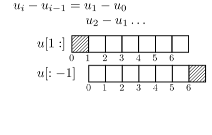
Figure 5:Array slices used to evaluate across the interior grid points. Adapted from Elhage (2015).
# Compute the solution using Euler's method and array slicing.
u = u0.copy()
for n in range(nt):
u[1:] = u[1:] - dt / dx * u[1:] * (u[1:] - u[:-1])# Plot the solution after nt time steps with the initial condition.
t_final = nt * dt
plt.figure(figsize=(3.0, 3.0))
plt.xlabel('x')
plt.ylabel('u')
plt.grid()
plt.plot(x, u0, label='Initial',
color='tab:blue', linestyle='--', linewidth=2)
plt.plot(x, u, label=f'FTBS, t = {t_final:.2f}',
color='tab:red', linestyle='-', linewidth=2)
plt.legend()
plt.xlim(0.0, L)
plt.ylim(0.0, 2.5);Hmm. That’s quite interesting: like in the linear case, we see that we have lost the sharp sides of our initial square wave, but there’s more. Now, the wave has also lost symmetry! It seems to be lagging on the rear side, while the front of the wave is steepening. Is this another form of numerical error, do you ask? No! It’s physics!
Same equation, different algorithms
The front of the wave steepens because larger values of move faster than smaller values. As that steepening produces a sharp jump, a choice that looked like ordinary algebra begins to matter numerically.
For a differentiable function, the chain rule gives
We can therefore write the nonlinear convection equation in conservative form:
As long as is smooth, Equation 16 and Equation 20 describe the same continuous equation. They do not, however, lead to the same discrete algorithm.
Discretize the two forms
The update used in the preceding computation applies a backward difference directly to ; we will call it the pointwise update. It is Equation 18. Applying the same forward-time, backward-space pattern to the flux derivative instead gives the conservative update:
The difference becomes visible by factoring the flux difference:
The pointwise update multiplies the backward difference by , while the conservative update effectively uses the average . When neighboring values are close, these multipliers become close under refinement. Across a jump, their difference is not small.
A balance built into the algorithm
The word conservative describes an algebraic property of the discrete update. Sum Equation 21 over the updated nodes :
Every interior flux appears once with a plus sign and once with a minus sign, so the sum telescopes: only the two boundary fluxes remain.
If we move the boundary-flux term in Equation 23 to the left and substitute a computed solution, the number left over is the discrete balance residual. More generally, a residual measures the amount by which computed values fail to satisfy an equation. For the conservative update, this residual is zero in exact arithmetic and should be close to zero in floating-point arithmetic. Over several time steps, we add the boundary contribution from each step and compare it with the total change from the initial state to the final state; the agent activity below calls this quantity the cumulative balance residual, . A small residual verifies this particular balance identity; it does not, by itself, prove that the flux or the rest of the implementation is correct.
If the endpoint fluxes are equal, the discrete total is unchanged apart from round-off. The pointwise update does not have this flux-difference structure and does not satisfy the same identity. This cancellation principle is central to conservative methods for nonlinear hyperbolic problems LeVeque, 2002.
When the solution remains differentiable, the chain rule supports the equivalence of the two continuous forms, and consistent discretizations should approach the same smooth solution. At a jump, the ordinary derivative used in the pointwise argument is no longer defined there, so that chain-rule argument is not enough to determine how the jump propagates. The conservative form retains a meaningful balance across the jump.
This short bridge does not yet develop the integral conservation law, weak solutions, shock speeds, or general numerical fluxes. Those ideas belong in Module 3. For now, the important warning is that algebraically equivalent smooth equations can produce algorithms with materially different behavior once discontinuities enter the computation.
On paper — compare one update
Before writing the two functions below, establish independent expectations:
Reproduce the chain-rule step leading to Equation 20, then derive Equation 21.
Let and , with the left value held fixed. Calculate one complete update using the pointwise formula and one using the conservative formula.
Expand the sum in Equation 23 for three updated nodes and cross out the canceling interior fluxes.
Predict what both updates should do to a constant array, and which update should satisfy the flux-balance identity to round-off.
Keep the two hand-calculated arrays nearby. They test the formulas and time levels directly, independently of the code.
In your notebook — implement both updates
Preserve your earlier direct computation. Then reconstruct the three small functions below in your notebook. Each step function must use only its arguments, leave its input array unchanged, hold the left boundary value fixed, and return a new array. Keep the names and argument order shown here because the agent-written diagnostic code will call this interface.
def nonlinear_flux(u):
    '''Return the quadratic flux for nonlinear convection.'''
    return 0.5 * u**2


def pointwise_step(u, dt, dx):
    '''Advance one step using the pointwise form.'''
    u_next = u.copy()
    u_next[1:] = (
        u[1:]
        - dt / dx * u[1:] * (u[1:] - u[:-1])
    )
    return u_next


def conservative_step(u, dt, dx):
    '''Advance one step using differences of the quadratic flux.'''
    u_next = u.copy()
    u_next[1:] = (
        u[1:]
        - dt / dx
        * (nonlinear_flux(u[1:]) - nonlinear_flux(u[:-1]))
    )
    return u_next
Check the functions against your hand calculation before asking an agent to build on them. The constant-state checks exercise a different property, so keep both kinds of evidence.
u_test = np.array([1.0, 2.0, 1.0])
pointwise_expected = np.array([1.0, 1.8, 1.1])
conservative_expected = np.array([1.0, 1.85, 1.15])

np.testing.assert_allclose(
    pointwise_step(u_test, dt=0.1, dx=1.0),
    pointwise_expected,
)
np.testing.assert_allclose(
    conservative_step(u_test, dt=0.1, dx=1.0),
    conservative_expected,
)
np.testing.assert_allclose(u_test, [1.0, 2.0, 1.0])

constant_test = np.full(5, 1.5)
np.testing.assert_allclose(
    pointwise_step(constant_test, dt=0.1, dx=1.0),
    constant_test,
)
np.testing.assert_allclose(
    conservative_step(constant_test, dt=0.1, dx=1.0),
    constant_test,
)
Compare the algorithms with an agent
The two update functions are short enough to derive, implement, and check yourself. Comparing them over several grids and tracking a flux balance is repetitive work that can usefully be delegated. The agent will first draft the comparison driver and later help you search for a blind spot in one diagnostic. In both roles, the agent proposes work for you to inspect; it will not choose the equations, change the algorithms, execute the code, or decide what the evidence means.
With an agent
Use an agent to add an unexecuted comparison driver to your own notebook. Allow it to inspect the notebook and add only the cells specified below. Do not allow changes to nonlinear_flux(), pointwise_step(), conservative_step(), earlier cells, or other files. Do not grant package-installation or network access.
You will inspect every added line before running one new cell at a time. The agent may organize the repetitive experiment; you remain responsible for the numerical specification, execution, audit, and conclusion.
Record expectations before delegation
In your notebook, record your answers to these questions before attaching it to an agent:
What maximum change do you expect after either function advances a constant state by one step?
What magnitude do you expect for the conservative scheme’s balance residual, obtained by moving all terms in Equation 23 to one side?
Does the pointwise update have an algebraic reason to produce the same residual?
As the grid is refined, should the two algorithms approach one another more clearly for the smooth hump or for the discontinuous square pulse? Why?
These are hypotheses to test, not outputs that the agent should be instructed to manufacture.
Use this bounded task brief
Add the following brief as a Markdown cell in your notebook. Read every requirement and resolve any mismatch with your own function names before delegating.
Agent algorithm-comparison task brief
Goal and scope: Add a comparison driver that compares my existing
pointwise_step()andconservative_step()functions. Do not implement, rewrite, or repair either method. Prefer named functions and straightforward, readable loops. The comparison concerns discrete behavior only; deriving shock speeds, introducing another scheme, and making the final numerical judgment are out of scope.Problem data: Use ,
nx_values = [81, 161, 321, 641, 1281], andt_compare = 0.15. For each grid, start with a targetdt = 0.2 * dx, round the step count to reach the common final time, and then resetdt = t_compare / num_stepsso every run ends at exactly the same time. Compare (a) the smooth hump and (b) the square pulse with background 1 and value 2 on . Each run must begin from a fresh copy of the same initial array.Required diagnostics: First report the maximum one-step change produced by each method from a constant array with value 1.5. Write a reusable runner named
run_balance_comparison(step_function, flux_function, initial_state, dt, dx, num_steps). It must return a dictionary containingu_final,initial_total,final_total,total_change, andbalance_residual.For every run, calculate these three diagnostics:
Here, is the discrete total, is the cumulative balance residual, and is the inter-algorithm difference at the final time. Evaluate for the initial and final states. In , use the boundary values from the state before each update. Evaluate using the two final solutions on the same grid.
Required output: Produce one readable table for each profile with
nx,dx, adjusteddt, step count, , both balance residuals, and both initial-to-final total changes. Produce a figure showing both final solutions on the finest grid for each profile and a log-log plot of against . Label methods, profiles, axes, and final time. Expose numerical values; do not replace them with pass/fail messages or a conclusion. Use only the NumPy and Matplotlib imports already present.Permissions and stopping rule: Inspect this notebook and add exactly three Python cells followed by one Markdown cell that records the added functions, experiment, plots, and any assumptions. Do not execute any cell, alter existing cells, write another file, install anything, or use the network. Stop after inserting those four cells and report that the comparison driver is ready for human audit.
Done when: The unexecuted cells contain the constant-state comparison, reusable balance runner, two-profile grid study, required tables and plots, plus the change record. An expected trend is not a completion condition; preserve and expose surprising results.
The brief separates the model and evidence you fixed from the code organization the agent may choose. Compare it with the minimum sufficient specification before granting access.
Invoke the agent
Save your notebook so the attachment contains your checked step functions, independent expectations, and task brief. Attach that notebook to your agent interface and send this short request:
Read the section titled “Agent algorithm-comparison task brief” in the attached notebook. Add the requested comparison driver and change record exactly as specified. Do not execute any cell or change existing work. Stop when the additions are ready for my audit.
If you do not have access to an agent that can edit a notebook, ask it to return the same four proposed cells in chat, add them yourself only after inspection, and follow the audit below.
Audit before execution
Inspect the notebook diff or the four inserted cells before running them. Confirm that the code:
calls your existing step functions without redefining or modifying them;
starts every method and grid from an independent copy of identical initial data;
uses the requested grids, profiles, and common physical time, and reports the adjusted
dtand step count;accumulates the boundary-flux term from the old state before each call to the step function;
uses the plus sign in the balance residual derived from Equation 23, with right-boundary flux minus left-boundary flux;
computes with the two solutions on the same grid and includes the factor ;
exposes totals and residuals for both methods rather than checking conservation only for the method named
conservative_step; andchanges no earlier cell or out-of-scope artifact.
If any item fails inspection, ask the agent to revise only its added cells, then inspect them again. Once the code passes, execute one inserted cell at a time. Recalculate one row’s and residual independently from the stored arrays. A clean plot or an agent statement that the method conserves is not a substitute for that arithmetic.
Test the diagnostics with known defects
A check that passes working code is not necessarily capable of detecting broken code. In this final exercise, you will challenge the diagnostics with two known defects and record which checks detect each one. Complete the steps in order, in new cells below the agent’s comparison driver.
First, save the accepted baseline results. Then add the two deliberately defective functions below under new names. Do not overwrite the correct functions. The first omits the factor in the intended flux; the second reads a newly updated left neighbor while marching across the array.
def conservative_step_missing_half(u, dt, dx):
    '''Deliberately use the wrong quadratic flux.'''
    u_next = u.copy()
    u_next[1:] = (
        u[1:] - dt / dx * (u[1:]**2 - u[:-1]**2)
    )
    return u_next


def pointwise_step_mixed_levels(u, dt, dx):
    '''Deliberately mix old and new time levels.'''
    u_next = u.copy()
    for i in range(1, u.size):
        u_next[i] = (
            u_next[i]
            - dt / dx * u_next[i]
            * (u_next[i] - u_next[i - 1])
        )
    return u_next
If you need to, review the Python refresher above that explained why the vectorized implementation of the spatial update is safe. The function pointwise_step_mixed_levels() is doing precisely what that admonition warned against: a “left-to-right” loop for the spatial update.
Step 1 — Check one update against known values
The earlier hand calculation gave the expected results for one update from with . Reuse those values as an independent reference. Add and run this code in a new notebook cell:
u_defect_test = np.array([1.0, 2.0, 1.0])
pointwise_expected = np.array([1.0, 1.8, 1.1])
conservative_expected = np.array([1.0, 1.85, 1.15])

missing_half_actual = conservative_step_missing_half(
    u_defect_test, dt=0.1, dx=1.0
)
mixed_levels_actual = pointwise_step_mixed_levels(
    u_defect_test, dt=0.1, dx=1.0
)

print('Missing-half result: ', missing_half_actual)
print('Expected conservative:', conservative_expected)
print('Mixed-level result:  ', mixed_levels_actual)
print('Expected pointwise:  ', pointwise_expected)

missing_half_detected = not np.allclose(
    missing_half_actual, conservative_expected
)
mixed_levels_detected = not np.allclose(
    mixed_levels_actual, pointwise_expected
)
assert missing_half_detected
assert mixed_levels_detected
The cell should run without an assertion error. Here, a passing assert means that the comparison successfully detected a mismatch. You should obtain [1.0, 1.7, 1.3] from the missing-half function and [1.0, 1.8, 1.08] from the mixed-level function.
Record: the known-value check detects both defects. For the mixed-level function, notice that the first updated value is correct; the error appears at the next point, after the loop reads the newly updated left neighbor: i=2 uses the updated value of u[1]. Follow the arithmetic on paper using the update of with .
Step 2 — Show what the constant-state check misses
Now apply both defective functions to a constant array. Add and run:
constant_defect_test = np.full(5, 1.5)

for method_name, step_function in (
    ('missing half', conservative_step_missing_half),
    ('mixed levels', pointwise_step_mixed_levels),
):
    actual = step_function(
        constant_defect_test, dt=0.1, dx=1.0
    )
    maximum_change = np.max(
        np.abs(actual - constant_defect_test)
    )
    print(f'{method_name:12s}: {maximum_change:.3e}')
    np.testing.assert_allclose(actual, constant_defect_test)
Both maximum changes should be zero, and both assertions should pass. This does not mean the functions are correct: every spatial difference is zero for a constant state, so neither defect is exercised.
Record: the constant-state check detects neither defect.
Step 3 — Use unequal boundary fluxes to detect the wrong flux
A conservative method may have a nonzero change in its discrete total when flux enters or leaves through the boundaries. The requirement is not total_change == 0; it is balance_residual == 0.
Use one step from an array whose endpoint values differ. The runner must receive the intended nonlinear_flux even when it calls the defective step function. Add and run:
u_balance_test = np.array([1.0, 2.0, 1.5])
balance_test_results = {}
for method_name, step_function in (
    ('conservative_step', conservative_step),
    (
        'conservative_step_missing_half',
        conservative_step_missing_half,
    ),
):
    balance_test_results[method_name] = run_balance_comparison(
        step_function, nonlinear_flux, u_balance_test.copy(),
        dt=0.1, dx=1.0, num_steps=1,
    )

print(f"{'method':>32} {'total change':>16} "
      f"{'balance residual':>20}")
for method_name, result in balance_test_results.items():
    print(
        f"{method_name:>32} "
        f"{result['total_change']:16.8e} "
        f"{result['balance_residual']:20.8e}"
    )
Before checking the output, calculate the intended boundary contribution:
The correct method should report total_change and a residual near zero. The missing-half method should report total_change and balance_residual . Confirm those expectations explicitly:
correct_balance = balance_test_results['conservative_step']
wrong_balance = balance_test_results[
    'conservative_step_missing_half'
]

np.testing.assert_allclose(
    correct_balance['total_change'], -0.0625, atol=1e-14
)
np.testing.assert_allclose(
    correct_balance['balance_residual'], 0.0, atol=1e-14
)
np.testing.assert_allclose(
    wrong_balance['total_change'], -0.125, atol=1e-14
)
np.testing.assert_allclose(
    wrong_balance['balance_residual'], -0.0625, atol=1e-14
)
Record: with unequal endpoint fluxes, the balance residual detects the missing factor . The correct total is not constant, but its change is fully explained by the boundary flux.
With an agent — red-team the balance residual
You have just shown that unequal endpoint fluxes make the wrong quadratic flux visible in the balance residual. Now ask an agent to look for a counterexample: a case in which that diagnostic passes even though the algorithm is still wrong.
Before contacting the agent, write one sentence predicting what would make the boundary-flux contribution lose its ability to distinguish the two fluxes. Then paste only the prompt below into the agent interface; do not attach the full notebook, because the next step contains the worked test.
I am checking a conservative update for the intended flux . A defective version uses . My diagnostic uses the intended flux:
With unequal endpoint values, detects the defect. Find a nonconstant initial state and a suitable run interval for which both the correct and defective updates could have near zero even though their final arrays differ. First identify the condition that the endpoint values must satisfy throughout the run, then explain your reasoning in no more than four bullets. Do not write or run code.
Treat the response as a hypothesis, not a result. Accept it only if it proposes a nonconstant state, explains why the endpoint condition should persist over the proposed interval, predicts what should happen to both residuals and the final arrays, and does not equate a zero residual with a correct implementation. Ask the agent to revise any missing or unsupported claim.
If you need a hint, ask: What relation between and makes , and how can you keep that relation true during a short run?
Record whether you accept, revise, or reject the agent’s proposed counterexample, and why. Then use Step 4 to test the proposal numerically.
Step 4 — Expose the balance check’s blind spot
Test the red-team hypothesis with a square pulse on a background of 1. This profile is nonconstant but has equal endpoint values. Use the coarsest grid from the agent study so the check runs quickly:
nx_square = 81
x_square = np.linspace(0.0, 2.0, num=nx_square)
dx_square = 2.0 / (nx_square - 1)
num_steps_square = int(round(0.15 / (0.2 * dx_square)))
dt_square = 0.15 / num_steps_square
u_square = np.ones(nx_square)
u_square[np.logical_and(x_square >= 0.5, x_square <= 1.0)] = 2.0

correct_square = run_balance_comparison(
    conservative_step, nonlinear_flux, u_square.copy(),
    dt_square, dx_square, num_steps_square,
)
wrong_square = run_balance_comparison(
    conservative_step_missing_half, nonlinear_flux,
    u_square.copy(), dt_square, dx_square, num_steps_square,
)
square_difference = dx_square * np.sum(
    np.abs(correct_square['u_final'] - wrong_square['u_final'])
)

print('Correct residual:   ',
      correct_square['balance_residual'])
print('Wrong-flux residual:',
      wrong_square['balance_residual'])
print('Difference between final states:', square_difference)

np.testing.assert_allclose(
    correct_square['balance_residual'], 0.0, atol=1e-12
)
np.testing.assert_allclose(
    wrong_square['balance_residual'], 0.0, atol=1e-12
)
assert not np.allclose(
    correct_square['u_final'], wrong_square['u_final']
)
Both residuals should be near zero even though the final arrays disagree; with these settings, square_difference is about . During this short run, the pulse remains separated from the boundaries and both endpoint values remain 1. The intended and incorrectly scaled fluxes therefore both have zero net boundary difference at every step. The global balance check cannot distinguish them in this case.
Record: the equal-endpoint square-pulse balance test misses the wrong flux. The nonzero solution difference shows disagreement, but without an independent reference it does not, by itself, identify which solution is correct.
Step 5 — Record what each diagnostic can detect
Add this completed detection table to your notebook beside the numerical output:
| Diagnostic | Missing | Mixed time levels |
|---|---|---|
| Known one-step values | Detected | Detected |
| Constant-state preservation | Not detected | Not detected |
| Unequal-boundary flux balance | Detected | Not applicable: the intended pointwise update is already nonconservative |
| Equal-endpoint square-pulse balance | Not detected | Not applicable |
Your conclusion should say that a passing diagnostic supports only the property and test case it actually exercises. The known-value check exposes both injected errors; the constant-state check exposes neither; and flux balance detects the wrong flux only when the boundary data make the discrepancy visible. No single passing check proves that an implementation is correct.
See Test the checks for the general role of this adversarial step.
Your verdict
Write a short debrief that answers:
Did you accept, revise, or reject the agent’s comparison driver? Name any change you made before execution.
Did both methods preserve a constant state? Report the measured maximum changes.
For each profile on the finest grid, report both balance residuals and explain what Equation 23 allows you to conclude.
Describe how changed under refinement for the smooth hump and square pulse. Does the evidence support treating the algorithms as interchangeable in both cases?
Which diagnostic caught each injected defect, and why was no single check sufficient? Did the agent’s proposed counterexample correctly identify a blind spot in the balance residual?
State what remains unresolved until the later conservation-law lesson; do not claim that this experiment derives a shock speed or proves general correctness.
Leave a lightweight agent record naming the agent or persona, the notebook attached for the first request, both prompts, permissions, cells and claims accepted or revised, and verification you performed.
Completion rubric
This is a Complete/Revise checkpoint. The activity is complete only when the specification, code audit, executed evidence, defect challenge, and learner judgment are all visible in your notebook.
| Criterion | Complete | Revise |
|---|---|---|
| Independent work | Both step functions pass hand-calculated and constant-state checks before delegation, and the learner predicts a possible blind spot before the red-team request. | The agent writes or repairs a numerical method, or expectations are accepted without independent reasoning. |
| Scope and access | The agent adds only the four unexecuted cells permitted by the first brief; the red-team request supplies only the bounded prompt. | Existing work changes, code is executed before audit, or either request receives broader access than needed. |
| Code audit | Checks common data, fresh state, time matching, flux timing and sign, totals, residuals, and . | Relies on names, plots, or the agent’s assurance instead of inspecting the calculation. |
| Evidence | Records the requested tables, plots, independent row calculation, and results from both profiles. | Reports only a visual impression or selected values that hide the comparison. |
| Adversarial check | Audits the agent’s proposed counterexample, runs both injected defects, and explains which diagnostics detect or miss each one. | Accepts the agent’s claim without testing it, or assumes passing baseline checks are effective without known faults. |
| Verdict and provenance | Makes a bounded claim, names unresolved theory, and records the agent interaction and human revisions. | Declares a generally correct method from this experiment or omits the agent record. |
What’s next?
The next lesson explains the stability restriction behind the failed fixed-dt refinement experiment. Module 3 will return to the conservative form from a control-volume balance, define how conservation laws represent discontinuous solutions, determine shock propagation, and apply those ideas to traffic flow.
- Elhage, N. (2015). Indices Point between Elements. https://blog.nelhage.com/2015/08/indices-point-between-elements/
- LeVeque, R. J. (2002). Finite Volume Methods for Hyperbolic Problems. Cambridge University Press. 10.1017/CBO9780511791253