The previous lessons are a great foundation in numerical methods for studying dynamical systems governed by ordinary differential equations. You learned to apply Euler’s method and studied its rate of convergence using numerical experiments. An exercise on paper in Lesson 2 using Taylor expansions showed that convergence to be first order. We found numerical evidence of this behavior in Lesson 3 using the full nonlinear phugoid model.
Euler’s method, however, showed a clear weakness for the undamped oscillator in Lesson 2: every step artificially increased its oscillation amplitude. You can understand this graphically. Each Euler step advances a variable (for example, position) to the next time interval using:
Recall that the derivative of a function corresponds to the slope of the tangent at a point. Euler’s method uses the slope at the initial point in an interval, and advances the numerical position with that initial velocity. In the sketch below we exaggerate the result: the Euler estimate overshoots the exact solution and the amplitude of the oscillation grows unphysically, adding a small amount of energy with every step.
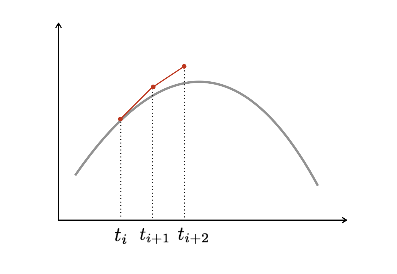
Figure 1:Sketch of two Euler steps approximating a curved time-dependent function.
First-order methods in general require very small time steps to achieve acceptable accuracy, and thus they are rarely used for real-world dynamical calculations. We now investigate a method with a higher order of accuracy. Among the most popular higher-order methods are the Runge-Kutta methods, developed around 1900: more than 100 years after Euler published his book containing the method now named after him.
Paper-airplane challenge
Throughout this lesson, we use this motivating challenge: how far can you make a paper airplane fly?
Once released, a paper airplane has no propulsion or active control; its flight depends strongly on the launch (angle and speed) and aerodynamic response. If we use computation to recommend a launch, we need to distinguish a genuine improvement from a change caused by time-stepping error.
Our engineering question is:
Find a competitive launch within specified bounds, then determine which method supports its predicted range to the required accuracy with less computational work.
You will use the following common problem data:
Model parameters: , (so ), , and . The lift-to-drag ratio is motivated by measurements reported by Feng & others (2009).
Release point: and . The release height is fixed.
Launch-search bounds: and . Convert angles to radians before using the model. These bounds define a model exercise, not experimentally validated launch limits.
Required numerical range accuracy: (1 cm). This is a target for the numerical calculation within the model, not a claim of centimeter accuracy for a real paper airplane.
Define range as the net horizontal displacement at the first crossing from positive altitude to nonpositive altitude. A run that has not reached the ground by the common time limit of 15 s, or encounters an invalid state, does not supply a usable range. This challenge is adapted from the computational phugoid exercise of Simanca & Sutherland (2002).
The investigation has two stages:
Controlled comparison: keep the launch fixed at and . Compare Forward Euler and explicit midpoint RK2 using the same ground-crossing procedure, then determine the work each needs to support the range-accuracy target. The comparison brief follows the convergence study.
Agent-supported launch investigation: search within the stated bounds of launch speed and angle, check that the best launches are not sensitive to the time step, test four nearby launches, then compare the methods for one competitive candidate. Treat ranges within 1 cm of the best tested range as equally useful for this exercise; the search does not prove a global optimum. The agent activity follows the controlled comparison.
Work through these stages in order. First derive and inspect the midpoint update, then reconstruct and verify the shared touchdown evaluator and complete the controlled comparison. In Stage 2, an AI agent may write the repetitive parameter-search code into your notebook, but you will inspect and execute each new cell yourself.
Runge–Kutta methods
A method’s order of convergence describes how the accumulated, or global, discretization error changes as we refine the time step over a fixed time interval. For a sufficiently smooth solution, a convergent method of order has global error . When the leading discretization-error term dominates, we expect approximately
where measures the global error and depends on the problem, method, and time interval, but not on . First-order error () scales linearly with the step size; second-order error () scales quadratically. These are small-step trends, not a guarantee that a higher-order method has a smaller error at every chosen step size.
One idea for improving on Euler’s method is to estimate the derivative at an intermediate point, like the midpoint, which results in the so-called explicit midpoint method or modified Euler method. The scheme has two steps and is written as:
Notice that this step evaluates the right-hand side, , twice: at the current state and at a predicted midpoint state. The notation represents an estimate of the state at . All Runge–Kutta methods use such intermediate evaluations, called stages. Their order depends on how the stage states are constructed and how the derivative evaluations are combined—not simply on how many evaluations are performed.
On paper — explain the midpoint update
First consider a scalar autonomous equation , with a sufficiently smooth . Start a single step from the exact value and use
Apply the chain rule to write . Expand and substitute it into Equation 3. Show that the numerical update matches Equation 4 through the terms in .
Explain why the midpoint state is a prediction, and why the final update must start from , not from that prediction.
Identify the one-step defect and explain why, under the smoothness and stability assumptions for convergence over a fixed interval, the accumulated error is second order.
When you reach rk2_step() below, check that both stages use complete state vectors. The scalar derivation motivates the construction; the implementation must advance all four components together.
Explicit midpoint is a second-order Runge–Kutta method (RK2). Its higher order does not eliminate all of Euler’s limitations. For the undamped oscillator in Lesson 2, sufficiently small time steps give less artificial amplitude growth than Forward Euler, but the amplitude still grows for any fixed, nonzero step size. Convergence as the step size shrinks over a fixed time interval is different from stable long-time behavior at a fixed step size.
An interesting historical connection to our phugoid problem: Carl Runge’s daughter Iris—an accomplished applied mathematician in her own right—worked assiduously over the summer of 1909 to translate Lanchester’s “Aerodonetics.” She also reproduced his graphical method to draw the phugoid curves Tobies, 2012, p. 73.
Phugoid model with second-order RK
Let’s begin the paper-airplane investigation by computing a baseline flight under the full phugoid model using both Forward Euler and second-order Runge–Kutta. We will use the same launch conditions for both methods and examine the horizontal distance traveled before the airplane touches the ground.
We will first compare the methods over a common interval while the airplane is still aloft. That fixed-time study checks the behavior of RK2, but it cannot yet justify a touchdown range or a time step for the engineering challenge. Afterward, we will build and verify the event calculation needed to measure range.
In your notebook
Create a new notebook for your work and keep this published lesson open as a worked reference. Reconstruct the midpoint update, the fixed-time refinement study, and the touchdown evaluator in your own notebook, including the direct first draft of the evaluator and the failure that motivates its checks. Type the numerical updates and event logic yourself so that you can connect each line to the equations; copying mechanical details such as imports, module-download code, and plot labels is fine.
Pause at each checkpoint. Record what you expect before running a cell, inspect the reported differences and statuses, and keep the steady-glide result as evidence that your reconstructed event calculation works. Consult Reconstruct a lesson for the general workflow.
Start by importing NumPy and Matplotlib with the aliases used in the previous lessons. We also set the font family and size through Matplotlib’s rcParams dictionary.
import numpy as np
import matplotlib.pyplot as plt
# Set the font family and size to use for Matplotlib figures.
plt.rcParams['font.family'] = 'serif'
plt.rcParams['font.size'] = 12Use the challenge’s lift-to-drag ratio and trim speed of . What do you think will happen if you make higher?
# Model parameters.
g = 9.81         # gravitational acceleration (m/s**2)
v_t = 4.9        # trim speed (m/s)
C_D = 1.0 / 5.0  # drag coefficient
C_L = 1.0        # lift coefficient

# Initial conditions.
v_0 = 6.5       # initial speed, above the trim speed (m/s)
theta_0 = -0.1  # trajectory angle (rad)
x_0 = 0.0       # horizontal position (m)
y_0 = 2.0       # altitude (m)
The initial speed is a little higher than the trim speed, the launch angle is negative, and the release height is 2 meters. We will use the same initial state and parameters for both numerical methods.
Reuse functions from a Python module
We have already written and inspected these three functions in Lesson 3:
rhs_full_phugoid()gives the four model derivatives.euler_step()advances the complete state by one Forward Euler step, in the*argsform.discrete_l1_difference()compares histories on nested time grids.
These functions are now reused often enough to save in a separate file. A module is an ordinary Python source file with the extension .py. To make one, create a plain-text file, copy the function definitions into it, and include the imports those definitions need—these functions only need import numpy as np. Keep parameter choices, integration loops, plots, and notebook-only commands in the notebook.
The course provides these definitions in a file named phugoid.py. Read the module source: its three functions are the ones already presented in previous lessons. We can download this file directly using urlretrieve() from Python’s standard library; add the code below to your notebook and execute it.
from urllib.request import urlretrieve

url = (
    'https://raw.githubusercontent.com/'
    'numerical-mooc/practical-numerical-methods/main/'
    'src/phugoid.py'
)
fname = 'phugoid.py'
urlretrieve(url, fname)
Here, url points to the raw Python file, and fname names the local copy. The file is saved in the kernel’s current working directory, normally the folder containing your notebook. Keep phugoid.py alongside your working notebook. You only need to download it once; rerunning the download overwrites that file, so save a separate copy of any local edits first.
Downloading saves the file; importing makes its functions available in the notebook. In the import statement, use the filename without .py. Python executes a module’s top-level statements when it first loads it, so you should only import code from sources you trust and have inspected. Our file imports NumPy and defines functions; it does not run a simulation.
Functions in the module do not inherit notebook variables, so we continue to pass the state and model parameters explicitly. The difference function requires both time-step sizes to check grid nesting and endpoint alignment.
If you edit the local module, restart the kernel and rerun your imports and calculations, skipping the download cell to preserve your edits. Rerunning an import alone does not reload an already imported module. For more detail, see the Python modules tutorial.
from phugoid import (
    discrete_l1_difference,
    euler_step,
    rhs_full_phugoid,
)
Define the RK2 step
The reused functions now come from the module, but the new numerical method stays visible here and in your notebook, as it is the first time you encounter it. Define rk2_step() to implement the modified Euler method in Equation 3, also known as second-order Runge–Kutta or RK2. The time loop will call this function once per step.
def rk2_step(u, f, dt, *args):
    '''Return the next state using the second-order Runge–Kutta method.

    Parameters
    ----------
    u : np.ndarray
        State at the current time
        as a 1D array of floats.
    f : function
        Function to compute the right-hand side of the system.
    dt : float
        Time-step size.
    *args
        Additional positional arguments passed to f.

    Returns
    -------
    u_new : np.ndarray
        The solution at the next time step
        as a 1D array of floats.
    '''
    u_star = u + 0.5 * dt * f(u, *args)
    u_new = u + dt * f(u_star, *args)
    return u_new
Compare on a common time interval
Begin with an illustrative time step of . We have not yet shown that this step is accurate enough for touchdown range, so do not treat it as an engineering recommendation. Integrate only to , when the baseline flight is still above ground, and compare the two approximations on exactly the same time grid.
As in Lesson 3, the variable num_steps counts updates; each history has num_steps + 1 rows to include the initial state. Both arrays have four columns ordered as [v, theta, x, y].
T_trajectory = 2.0  # common pre-impact interval (s)
dt = 0.01  # time-step size (s)
num_steps = int(round(T_trajectory / dt))

# Store the state at every time point, including the initial state.
u_euler = np.empty((num_steps + 1, 4))
u_rk2 = np.empty((num_steps + 1, 4))
u_euler[0] = np.array([v_0, theta_0, x_0, y_0])
u_rk2[0] = np.array([v_0, theta_0, x_0, y_0])

# Advance both methods over the same time grid.
for n in range(num_steps):
    u_euler[n + 1] = euler_step(
        u_euler[n], rhs_full_phugoid, dt, C_L, C_D, g, v_t
    )
    u_rk2[n + 1] = rk2_step(
        u_rk2[n], rhs_full_phugoid, dt, C_L, C_D, g, v_t
    )
Extract time, horizontal position, and altitude for the exploratory plot. The final altitudes will also confirm that this entire comparison ends before impact.
# Extract the common time grid and both position histories.
t_trajectory = np.linspace(0.0, T_trajectory, num_steps + 1)
x_euler = u_euler[:, 2]
y_euler = u_euler[:, 3]
x_rk2 = u_rk2[:, 2]
y_rk2 = u_rk2[:, 3]
print(f'Final Euler altitude: {y_euler[-1]:.3f} m')
print(f'Final RK2 altitude:   {y_rk2[-1]:.3f} m')
Plot for exploration, not an accuracy test
A trajectory plot is a useful first diagnostic: it can expose a wrong sign, a discontinuity, or an implausible path. It cannot show that a range is accurate to 1 cm. Two curves can overlap visually while differing by more than the required tolerance.
For now, inspect the two paths and their separation. This is exploratory evidence, not a verdict.
fig, axes = plt.subplots(1, 2, figsize=(9.0, 4.0))
for ax in axes:
    ax.grid()
    ax.set_xlabel('Horizontal position, x (m)')
    ax.set_ylabel('Altitude, y (m)')

# Plot both approximations over the common pre-impact interval.
axes[0].plot(x_euler, y_euler, label='Euler')
axes[0].plot(x_rk2, y_rk2, label='RK2')
axes[0].legend()

# Plot their horizontal separation on the same time grid.
axes[1].plot(t_trajectory, x_rk2 - x_euler)
axes[1].set_xlabel('Time, t (s)')
axes[1].set_ylabel(r'$x_{RK2} - x_{Euler}$ (m)')
fig.tight_layout()
Fixed-time trajectory convergence
Just like in Lesson 3, we want to check whether RK2 exhibits its expected convergence rate on this problem. Every history below ends at the same pre-impact time, , so values at matching indices describe the same physical times.
The for loop computes the solution on several nested time grids, with the coarsest and finest step sizes differing by a factor of 100. We then compare horizontal position, a single quantity with units of meters. Mixing all four state columns would combine speed, angle, horizontal position, and altitude in one number with no coherent physical units.
# Set the time-step sizes to investigate.
dt_values = [0.1, 0.05, 0.01, 0.005, 0.001]
u_histories = []

for dt_trial in dt_values:
    num_steps_trial = int(round(T_trajectory / dt_trial))
    u_trial = np.empty((num_steps_trial + 1, 4))
    u_trial[0] = np.array([v_0, theta_0, x_0, y_0])

    for n in range(num_steps_trial):
        u_trial[n + 1] = rk2_step(
            u_trial[n], rhs_full_phugoid, dt_trial,
            C_L, C_D, g, v_t,
        )
    u_histories.append(u_trial)
For the general nonlinear trajectory computed here, we do not have an exact reference solution available. The finest-grid history is a numerical reference, not an exact solution, so the differences below are not exact errors. They are evidence about refinement behavior over this fixed interval.
Once those runs are complete, compare each horizontal-position history with the finest-grid history. Pass both time-step sizes to the imported discrete_l1_difference() function so it can align the grids.
# Compute the differences in horizontal position.
difference_values = []
for u_trial, dt_trial in zip(u_histories, dt_values, strict=True):
    difference = discrete_l1_difference(
        u_trial[:, 2], u_histories[-1][:, 2],
        dt_trial, dt_values[-1],
    )
    difference_values.append(difference)
Plot the differences against time-step size on logarithmic axes, as in the previous lessons.
fig, ax = plt.subplots(figsize=(5.0, 5.0))
ax.set_title(r'$L_1$ difference vs. time-step size')
ax.set_xlabel(r'$\Delta t$ (s)')
ax.set_ylabel(r'$L_1$ difference in $x$')
ax.grid()
ax.loglog(
    dt_values[:-1], difference_values[:-1],
    color='tab:blue', linestyle='--', marker='o',
)
ax.set_aspect('equal', adjustable='box')
fig.tight_layout()
The decreasing differences suggest convergence, but their size is measured relative to a numerical reference. In Lesson 3, the observed order for Euler’s method was close to 1. For RK2, the expectation is once the leading discretization-error term dominates. Let us test that expectation.
To compute the observed order of convergence, we use three grid resolutions that are refined at a constant rate, in this case .
refinement_ratio = 2
dt_fine = 0.001
dt_order = [
    dt_fine,
    refinement_ratio * dt_fine,
    refinement_ratio**2 * dt_fine,
]
u_order = []

for dt_trial in dt_order:
    num_steps_trial = int(round(T_trajectory / dt_trial))
    u_trial = np.empty((num_steps_trial + 1, 4))
    u_trial[0] = np.array([v_0, theta_0, x_0, y_0])

    for n in range(num_steps_trial):
        u_trial[n + 1] = rk2_step(
            u_trial[n], rhs_full_phugoid, dt_trial,
            C_L, C_D, g, v_t,
        )
    u_order.append(u_trial)

# Compare horizontal position on the three grids.
difference_coarse_medium = discrete_l1_difference(
    u_order[2][:, 2], u_order[1][:, 2],
    dt_order[2], dt_order[1],
)
difference_medium_fine = discrete_l1_difference(
    u_order[1][:, 2], u_order[0][:, 2],
    dt_order[1], dt_order[0],
)
difference_ratio = difference_coarse_medium / difference_medium_fine
observed_order = (
    np.log(difference_ratio) / np.log(refinement_ratio)
)

print(f'Coarse–medium difference: {difference_coarse_medium:.6e} m s')
print(f'Medium–fine difference:   {difference_medium_fine:.6e} m s')
print(f'Difference ratio:         {difference_ratio:.3f}')
print(f'Observed order:           p = {observed_order:.3f}')
An observed order close to 2 is consistent with the expected second-order behavior for this grid family. In the regime where the leading error is proportional to , halving the step size reduces that error to approximately one quarter of its previous size. The raw differences and their ratio make that conclusion inspectable rather than reporting only the final value of .
This study concerns horizontal-position histories over a fixed, airborne interval. It does not verify touchdown range or justify for the challenge. Touchdown occurs at a step-dependent time, and locating it introduces a separate event-calculation error. We need to define and test that measurement before studying range convergence.
Locate touchdown and evaluate range
Touchdown is an event: it happens when the altitude first crosses the ground, not necessarily at one of our stored times. Starting from positive altitude, one numerical step brackets touchdown when
Assume the state changes linearly between those two computed endpoints. Let be the fraction of the step needed to reach . Linear interpolation gives
Because the two altitudes bracket zero, . The horizontal component of supplies the interpolated touchdown position, and the net range is . We retain the two computed endpoints as the crossing bracket, but stop immediately: no later below-ground states are calculated.
A usable result also needs an explicit completion status. We will report touchdown, time_limit, or invalid_state; the third arises when a calculation breaks, and we will see below why it needs a status of its own. Failed or unfinished runs receive no range.
On paper — interpolate one crossing
A step from to takes the altitude from to , the horizontal position from to , and the speed from 6.0 to .
Compute from Equation 6 and confirm that .
Compute the touchdown time , the horizontal position , and the speed at touchdown.
Explain why the interpolated altitude must be exactly zero.
Keep these values: they become the expected values in a test below.
Write the interpolation as a function
The crossing formula is small enough to be its own function, so that we can test it by hand before it is buried inside a loop. locate_touchdown() receives the two times and states that bracket the crossing and returns the interpolated touchdown time and state.
def locate_touchdown(t, u, t_next, u_next):
    '''Interpolate the ground crossing inside one bracketing step.

    Parameters
    ----------
    t, t_next : float
        Times at the start and end of the bracketing step.
    u, u_next : np.ndarray
        States at those times, with u[3] > 0 and u_next[3] <= 0.

    Returns
    -------
    t_touchdown : float
        Interpolated time of the crossing.
    u_touchdown : np.ndarray
        Interpolated state at the crossing.
    '''
    alpha = u[3] / (u[3] - u_next[3])
    t_touchdown = t + alpha * (t_next - t)
    u_touchdown = u + alpha * (u_next - u)
    return t_touchdown, u_touchdown
Check the function against your hand calculation before using it. The bracket below uses the values from the On paper exercise; the expected values come from that calculation, not from the code.
u_above = np.array([6.0, -0.2, 5.0, 0.3])
u_below = np.array([6.1, -0.2, 5.06, -0.1])
t_check, u_check = locate_touchdown(2.0, u_above, 2.01, u_below)

np.testing.assert_allclose(t_check, 2.0075)
np.testing.assert_allclose(u_check, [6.075, -0.2, 5.045, 0.0])
Start with a direct loop
Before adding any checks, write the range calculation directly: take a step, test for a crossing, interpolate, and stop. If the flight is still aloft when the steps run out, report that instead. A for loop over int(np.floor(time_limit / dt)) takes only complete steps within the safety cap; ending less than one step early is harmless here. The function returns a status and a range, and the status time_limit means that no crossing was found.
def range_first_draft(step_function, u_0, f, dt, time_limit, *args):
    '''Return a status and range from a loop with no validity checks.'''
    u = np.asarray(u_0, dtype=float)
    x_initial = u[2]
    for n in range(int(np.floor(time_limit / dt))):
        u_next = step_function(u, f, dt, *args)
        if u_next[3] <= 0.0:
            t_touchdown, u_touchdown = locate_touchdown(
                n * dt, u, (n + 1) * dt, u_next
            )
            return 'touchdown', u_touchdown[2] - x_initial
        u = u_next
    return 'time_limit', None
Apply this function to the baseline launch, then to a launch with zero initial speed. The model contains , so zero speed is outside its domain. Predict what the function will report in the second case before running the cell.
u_baseline = np.array([v_0, theta_0, x_0, y_0])
print(range_first_draft(
    euler_step, u_baseline, rhs_full_phugoid, 0.01, 15.0, C_L, C_D, g, v_t
))

u_zero_speed = np.array([0.0, theta_0, x_0, y_0])
print(range_first_draft(
    euler_step, u_zero_speed, rhs_full_phugoid, 0.01, 15.0, C_L, C_D, g, v_t
))
A silent wrong answer
The first result is the interpolated baseline range. The second is wrong in a way that is easy to miss. NumPy printed a warning about division by zero, but a warning does not stop a calculation. The first step produced an infinite trajectory angle, and the following step turned the state into nan, which stands for “not a number.” Every comparison with nan is False, including u_next[3] <= 0.0, so the crossing test never fires and the loop runs to the time limit. The draft function then reports that the airplane never landed, when in fact the calculation broke on its first step. Confirm the behavior of the comparison:
print(np.nan <= 0.0, np.nan > 0.0, np.isfinite(np.nan))
A result that looks like a legitimate outcome, time_limit, but comes from a broken calculation is a type of failure that needs to be prevented with defensive checks. The remedy is a validity test on every completed step, placed before the crossing test, so that a broken state is reported as such rather than silently compared. A state is valid when every entry is finite and the speed is positive: negative speed is outside the state convention, and zero speed is outside the model’s domain. A nonpositive altitude reached from a positive altitude is the event, not an invalid state.
We can write this test as a small function and check it on a valid state, the zero-speed state, and a state containing nan.
def state_is_valid(u):
    '''Return True when every entry is finite and the speed is positive.'''
    return np.all(np.isfinite(u)) and u[0] > 0.0


assert state_is_valid(u_baseline)
assert not state_is_valid(u_zero_speed)
assert not state_is_valid(np.array([np.nan, theta_0, x_0, y_0]))
Map the possible outcomes
Before any more coding, you should understand the possible outcomes. The complete evaluator has four jobs:
Check the setup. A nonpositive time step, an initial state with the wrong number of entries, or a nonpositive initial altitude is a caller error: no crossing from positive altitude could ever be found, and the draft function above would silently report
time_limit. The full function raisesValueErrorrather than starting a calculation with a broken setup.Advance and count steps. The evaluator counts accepted completed steps, including the step that brackets touchdown. A step that first exposes an invalid state is rejected and not counted; failed runs do not enter the work comparison. For successful runs, multiplying by one right-hand-side evaluation per Euler step or two per midpoint step gives the computational work.
Recognize a failed flight calculation. A completed step whose state is non-finite or has nonpositive speed produces the status
invalid_stateand no range. The check inspects completed steps only; a stricter evaluator would also inspect RK2’s intermediate stage.Recognize completion. The first positive-to-nonpositive altitude bracket produces
touchdown; using up the steps without such a bracket producestime_limit. Only touchdown supplies a range.
Here is the same control flow as pseudocode. Read this outline first, then find each part in the Python function below.
check the setup

for each step up to the time limit:
    take one numerical step
    if the new state is invalid:
        stop with invalid_state
    store the new state
    if altitude crossed zero:
        interpolate touchdown
        stop with touchdown

report time_limit
At the start of the function, np.asarray(u_0, dtype=float) normalizes a list or array into floating-point NumPy data. We call that working state u because it changes as the integration advances, while u_0 names the original initial condition. The initial horizontal position is saved separately so the final range can always be measured from the launch point.
def integrate_until_touchdown(
    step_function, u_0, f, dt, time_limit, *args
):
    '''Integrate until touchdown, the time limit, or an invalid state.'''
    if dt <= 0.0:
        raise ValueError('dt must be positive.')

    u = np.asarray(u_0, dtype=float)
    if u.shape != (4,) or u[3] <= 0.0:
        raise ValueError(
            'u_0 must contain [v, theta, x, y] with positive altitude.'
        )
    x_initial = u[2]

    max_steps = int(np.floor(time_limit / dt))
    times = [0.0]
    states = [u.copy()]
    status = 'time_limit'
    touchdown_time = None
    touchdown_state = None
    range_value = None

    for n in range(max_steps):
        u_next = step_function(u, f, dt, *args)

        if not state_is_valid(u_next):
            status = 'invalid_state'
            break

        t_next = (n + 1) * dt
        times.append(t_next)
        states.append(u_next)

        if u_next[3] <= 0.0:
            touchdown_time, touchdown_state = locate_touchdown(
                n * dt, u, t_next, u_next
            )
            range_value = touchdown_state[2] - x_initial
            status = 'touchdown'
            break

        u = u_next

    return {
        'status': status,
        'times': np.asarray(times),
        'states': np.asarray(states),
        'touchdown_time': touchdown_time,
        'touchdown_state': touchdown_state,
        'range': range_value,
        'steps': len(times) - 1,
    }
Check the non-success outcomes
A failure path deserves a test just as much as a successful calculation. Use a deliberately short time limit to produce an unfinished run, then supply the zero-speed launch that fooled the first draft of the evaluator. In both cases, inspect the status and confirm that range is unavailable. The zero-speed run now rejects its first attempted step instead of running to the time limit; its reported steps value is therefore zero.
unfinished_result = integrate_until_touchdown(
    euler_step, u_baseline, rhs_full_phugoid,
    0.01, 0.1, C_L, C_D, g, v_t,
)
invalid_result = integrate_until_touchdown(
    euler_step, u_zero_speed, rhs_full_phugoid,
    0.01, 15.0, C_L, C_D, g, v_t,
)

for result in (unfinished_result, invalid_result):
    print(
        f'{result["status"]}: range = {result["range"]}; '
        f'{result["steps"]} accepted steps'
    )

assert unfinished_result['status'] == 'time_limit'
assert unfinished_result['range'] is None
assert unfinished_result['steps'] == 10
assert invalid_result['status'] == 'invalid_state'
assert invalid_result['range'] is None
assert invalid_result['steps'] == 0
The initial-state guard also deserves a test. The cell below deliberately passes a release point below ground (-1.0) and confirms that the function refuses to start. It is a small test asking: “Does the function refuse to simulate an aircraft that already starts below ground?” The draft evaluator would have treated the first update as touchdown because its altitude was already nonpositive. With both endpoints below ground, locate_touchdown() would extrapolate to a fictitious crossing outside the step rather than interpolate a real bracket.
u_below_ground = np.array([v_0, theta_0, x_0, -1.0])
guard_triggered = False
try:
    integrate_until_touchdown(
        euler_step, u_below_ground, rhs_full_phugoid,
        0.01, 15.0, C_L, C_D, g, v_t,
    )
except ValueError as error:
    guard_triggered = True
    print('Rejected:', error)

assert guard_triggered
The invalid input is created with -1.0 on the last element of u_below_ground. The test begins by assuming the guard has not run:
guard_triggered = FalseThen it tries to call the function:
try:
    integrate_until_touchdown(...)
Inside the function, this condition detects the negative altitude:
if u.shape != (4,) or u[3] <= 0.0:
    raise ValueError(...)
Normally that would stop the cell. However, the except block catches that particular error, and guard_triggered = True records that the expected rejection occurred. The final assert checks that the function really did reject the input.
The complete flow is:
Negative altitude supplied
        ↓
Function raises ValueError
        ↓
except catches it
        ↓
guard_triggered becomes True
        ↓
assert passes
Reread this little test and explanation as many times as you need. Check your understanding by answering: what would happen if the altitude check were accidentally removed?
Verify the evaluator with steady glide
The general nonlinear flight lacks an exact solution we can use to verify the evaluator, but the model does have an exact steady-glide special case.
On paper — confirm exact special case
Set and in the model equations. With , show that the descending equilibrium has
The steady-glide speed is not exactly the trim-speed parameter . Use the constant derivatives and to eliminate time and show that the range from height is
Use as a separate verification initial state, not as a replacement for the baseline launch. Because the vertical velocity is constant, the exact touchdown time is . Both Euler and RK2 advance this straight-line motion exactly apart from floating-point effects.
The step sizes below place touchdown strictly between stored times. For every trial, require the touchdown status, confirm that the interpolated time lies inside the final bracket, and compare the range with Equation 8. This checks the event calculation; it does not establish accuracy for a curved trajectory or validate the physical model.
eta = C_D / C_L
theta_steady = -np.arctan(eta)
v_steady = v_t * np.sqrt(np.cos(theta_steady))
u_steady = np.array([v_steady, theta_steady, 0.0, y_0])
exact_steady_time = -y_0 / (v_steady * np.sin(theta_steady))
exact_steady_range = y_0 * C_L / C_D
verification_dts = [0.5, 0.4, 0.25]

print('method      dt (s)   touchdown (s)   range (m)   error (m)')
for method_name, step_function in (
    ('Euler', euler_step), ('RK2', rk2_step)
):
    for dt_trial in verification_dts:
        result = integrate_until_touchdown(
            step_function, u_steady, rhs_full_phugoid,
            dt_trial, 15.0, C_L, C_D, g, v_t,
        )
        assert result['status'] == 'touchdown'
        range_error = abs(result['range'] - exact_steady_range)
        print(
            f'{method_name:<8} {dt_trial:8.2f} '
            f'{result["touchdown_time"]:15.9f} '
            f'{result["range"]:11.9f} {range_error:11.3e}'
        )

        assert (
            result['times'][-2]
            < result['touchdown_time']
            < result['times'][-1]
        )
        assert abs(result['touchdown_time'] - exact_steady_time) < 1e-10
        assert range_error < 1e-10
The assertions are deliberately demanding because this equilibrium produces straight-line motion: the time-stepping methods and the linear event model are exact for this case apart from floating-point rounding. Passing this test at several off-grid touchdown times gives us a focused check of the bracketing and interpolation logic. It does not tell us how small must be for the curved baseline flight; that requires range refinement.
Compare methods at a required accuracy
This is Stage 1 of the paper-airplane challenge. Keep the baseline launch and all model parameters fixed. The question is not which method runs faster on the same grid, but which needs fewer right-hand-side evaluations to support a range accurate to 1 cm.
We now have a verified range evaluator with explicit completion statuses and a common event treatment for both methods. Our next goal is to apply it first to the baseline launch at the illustrative step size, then establish a numerical reference by refinement.
Apply the evaluator to the baseline launch
Return to the baseline initial state and use the illustrative step size . The next cell demonstrates the evaluator’s interface and confirms that each successful run stops at its first crossing bracket. The printed ranges are interpolated, but they are still provisional numerical results: we have not yet established their errors by refinement.
dt_touchdown = 0.01
time_limit = 15.0
rhs_calls_per_step = {'Euler': 1, 'RK2': 2}
flight_results = {}

for method_name, step_function in (
    ('Euler', euler_step), ('RK2', rk2_step)
):
    result = integrate_until_touchdown(
        step_function, u_baseline, rhs_full_phugoid,
        dt_touchdown, time_limit, C_L, C_D, g, v_t,
    )
    flight_results[method_name] = result
    work = result['steps'] * rhs_calls_per_step[method_name]

    if result['range'] is None:
        print(
            f'{method_name}: {result["status"]}; '
            f'range unavailable; {work} RHS evaluations'
        )
    else:
        print(
            f'{method_name}: {result["status"]}; '
            f't = {result["touchdown_time"]:.6f} s; '
            f'R = {result["range"]:.6f} m; '
            f'{work} RHS evaluations'
        )
fig, ax = plt.subplots(figsize=(6.0, 4.0))
for method_name, result in flight_results.items():
    path = result['states'].copy()
    if result['status'] == 'touchdown':
        # Replace the below-ground bracket endpoint by the event point.
        path[-1] = result['touchdown_state']
    ax.plot(path[:, 2], path[:, 3], label=method_name)

ax.set_xlabel('Horizontal position, x (m)')
ax.set_ylabel('Altitude, y (m)')
ax.grid()
ax.legend()
fig.tight_layout()
For a successful run, states contains the two endpoints that bracket touchdown. The plotting cell keeps the last valid computed point but replaces the nonpositive endpoint with touchdown_state, so the displayed physical path ends at . Work is counted in right-hand-side evaluations: the completed steps, including the bracketing step, multiplied by one evaluation per Euler step or two per midpoint step. The dictionary rhs_calls_per_step records those factors so that the conversion stays visible.
The two methods are not required to use the same time step in the final engineering comparison. Equal is a useful diagnostic, but it gives RK2 about twice the computational work while its computational accuracy is superior. Our primary question is thus: what is the least RHS work each method needs to support the same range accuracy?
Establish a numerical range reference
The baseline ranges at one time step are provisional. Without an exact solution for the curved flight, the reference is a refined RK2 result, accepted when the range changes by less than one tenth of the accuracy target, 1 mm, in each of two successive step halvings. A reference must be resolved well beyond the tolerance it will be used to judge; this rule provides evidence of that, not a rigorous error bound. The cell below applies the rule starting from and stops at the first step size that satisfies it, or reports insufficient evidence after eight halvings. It also adds up the work spent on the reference, which is reported separately from the comparison itself, and it stores the accepted range as range_reference and its step size as dt_search, the names used by the comparison below and by Stage 2.
range_target = 0.01  # required numerical range accuracy (m)
reference_tolerance = 0.1 * range_target  # a reference must beat the target
dt_reference = dt_touchdown
result = integrate_until_touchdown(
    rk2_step, u_baseline, rhs_full_phugoid,
    dt_reference, time_limit, C_L, C_D, g, v_t,
)
range_previous = result['range']
reference_work = result['steps'] * rhs_calls_per_step['RK2']
small_changes = 0
reference_accepted = False

print('dt (s)         range (m)    change (m)')
print(f'{dt_reference:<12.6f} {range_previous:12.6f}')
for halving in range(8):
    dt_reference = dt_reference / 2
    result = integrate_until_touchdown(
        rk2_step, u_baseline, rhs_full_phugoid,
        dt_reference, time_limit, C_L, C_D, g, v_t,
    )
    assert result['status'] == 'touchdown'
    reference_work += result['steps'] * rhs_calls_per_step['RK2']
    change = abs(result['range'] - range_previous)
    print(f'{dt_reference:<12.6f} {result["range"]:12.6f} {change:12.3e}')
    range_previous = result['range']

    if change < reference_tolerance:
        small_changes += 1
    else:
        small_changes = 0
    if small_changes == 2:
        reference_accepted = True
        break

assert reference_accepted, 'Insufficient evidence for a range reference.'
range_reference = range_previous
dt_search = dt_reference
print(f'Reference range: {range_reference:.6f} m at dt_search = {dt_search:g} s')
print(f'Work to establish the reference: {reference_work} RHS evaluations')
The two successive step halvings changed the RK2 range by less than 1 mm each, so we accept the last result as our working numerical reference. The cell stores that range as range_reference and its step size as dt_search; use these variables, rather than retyped values, in the accuracy-and-work comparison and in Stage 2.
In your notebook, also refine Euler and check that its ranges move toward range_reference, continuing until their difference is well inside the 1 cm target. Euler is first-order, so expect more halvings. The results need not agree in every printed digit: both retain discretization error. Do not assign to range_reference or dt_search in the Euler check, so that the RK2 values are not overwritten.
Plan the accuracy-and-work comparison
Which method needs fewer right-hand-side (RHS) evaluations for a range accurate to 1 cm? Reuse your existing functions, keeping the baseline launch, model parameters, touchdown interpolation, and 15 s time limit fixed.
Keep one shared reference. Use
range_reference, the accepted RK2 range, as for both methods; your Euler cross-check plays no part in it.Build a table of runs. For each method, start at and halve the step at least three times: 0.05, 0.025, and . Continue halving as needed. Starting coarse reveals where each method becomes accurate enough.
Find and check a qualifying run. A run qualifies when , the accuracy target. After finding one, halve the step at least once more and check that the finer run still qualifies and its difference from the reference decreases. Otherwise, investigate and refine further.
Compare work. For each method, select the least-work qualifying run supported by the finer-step check. The selected runs may use different time steps.
Record one row per run, replacing the dashes and extending this table as needed:
| Method | Time step (s) | Range (m) | Absolute difference from reference (m) | RHS evaluations | Status |
|---|---|---|---|---|---|
| Euler | 0.1 | — | — | — | — |
| Euler | 0.05 | — | — | — | — |
| … | … | … | … | … | … |
| RK2 | 0.1 | — | — | — | — |
| RK2 | 0.05 | — | — | — | — |
| … | … | … | … | … | … |
For each row, compute work as result['steps'] * rhs_calls_per_step[method_name]. Count only that run. For failed or unfinished runs, record None for both range and difference, keep status and work, and exclude them from selection. Report the accumulated RK2 reference work and Euler cross-check work separately below the table.
Plot the absolute difference from the reference against RHS evaluations, using a logarithmic scale on both axes and a horizontal line at . These differences are not exact errors.
Conclude with each method’s selected step size, work count, and supporting refinement. State which uses less work and by what factor, for this baseline and tested steps. If evidence is insufficient, say so.
Together with your earlier derivations, touchdown verification, and reference checks, this table, plot, and conclusion complete Stage 1.
Investigate launches with an agent
We return to the motivating question: which launch flies farthest, and which method supports its predicted range with less work? You now have a verified touchdown evaluator, an accepted search step dt_search, and a procedure for comparing the two methods at 1 cm accuracy. What remains is repetitive: hundreds of runs over a grid of launch speeds and angles. An agent will write that code into your notebook. You will read each cell before running it, run it yourself, and decide what the results mean.
Two ideas guide the whole activity. Keep them in mind while you read the agent’s output.
Treat launches within 1 cm of the best tested range as tied for our recommendation. We choose not to distinguish smaller improvements for this paper-airplane exercise. This is an engineering judgment about useful precision, even when the numerical calculation resolves smaller differences; it does not establish the accuracy of the model for a real airplane.
A time step is validated for a flight, not for a method. Stage 1 found the time step each method needs for the 6.5 m/s launch. The best launches fly faster and farther, so you can expect they could need smaller steps. The last part of the activity measures this.
The search uses dt_search, the step accepted for the range reference, rather than the coarser step that met the 1 cm target in Stage 1. This better-resolved step helps keep numerical error small compared with our 1 cm decision threshold.
With an agent
Work in your own notebook. The agent adds code cells; you audit and run them yourself. The activity has four steps:
| Step | Who | What |
|---|---|---|
| 1. Search | Agent writes, you run | The range of every launch on a grid, and the five best |
| 2. Check | Agent writes, you run | Halve the time step for the five best; test four nearby launches |
| 3. Choose | You | List competitive launches, choose one, and establish its reference range |
| 4. Compare | Agent writes, you run | Euler and RK2 computational work for that launch at 1 cm accuracy |
Both briefs are supplied, so that you can concentrate on auditing. They use the four headings from the agent-use guide.
Record the launch-search brief
Copy the brief below into a Markdown cell in your notebook and fill in the two bracketed entries. Above it, note the date and the agent or persona you use.
Agent launch-search task brief
Goal and scope
Add two readable, unexecuted Python cells below this brief in [notebook filename]. Cell 1 searches a grid of launches. Cell 2 checks the leading launches. Leave the choice of launch and all conclusions to me.
Non-negotiables
Reuse rk2_step(), rhs_full_phugoid(), integrate_until_touchdown(), the model parameters, the release point, and the 15 s time limit already in the notebook. Use the notebook variable dt_search, whose value is [accepted RK2 step]. Use ordinary loops and comments. Report angles in degrees and convert to radians only when building a state.
Cell 1, the search:
Run RK2 at
dt_searchfor all 17 equally spaced speeds from 4 to 12 m/s and all 25 equally spaced angles from to , endpoints included: 425 launches.Keep one record per launch: speed, angle in degrees, range, status, and step count. A failed or unfinished run keeps
range=Noneand is never ranked.Print the count of each status, then the five largest ranges with their speed and angle. Keep all records in a list for Cell 2. If fewer than five runs succeed, print that instead and stop.
Cell 2, the checks:
Time step: rerun the five best launches at
dt_search/2. For each, print the range and status at both steps and the change between successful results.Nearby launches: around the best launch from Cell 1, change only the angle by and , then only the speed by -0.25 and +0.25 m/s. Skip any point outside the original bounds. Run these checks at
dt_search/2. Print each range and its signed change from the center launch at that same step; positive means farther.Retain all check records and statuses. Failed or unfinished checks keep
Nonefor range and change.Print results only. Do not rank, choose, or comment on them.
Allowed actions
Read the attached notebook and add only these two cells. The following are disallowed: changing existing cells, redefining the model or numerical functions, running code, creating files, downloading anything, accessing the network, or installing packages.
Done when
Both cells are inserted, without outputs or execution counts. Stop and report where they were added and which variables they create. I will inspect and run them.
Invoke the agent
Save the notebook with your completed brief and attach it to your agent interface. If the interface lets you allow edits but not execution, set it that way. Send this short request:
Read “Agent launch-search task brief” in the attached notebook and add the requested cells. Follow its allowed actions and return only the requested change record.
Audit and run the search
Audit — before you run anything
Read the agent’s report and look at the notebook. Earlier cells must be unchanged, and the new cells must have no outputs. Then read the code against the brief:
Does Cell 1 cover all 425 launches, include both endpoints of each range, and convert degrees to radians?
Do both cells call your existing functions rather than new versions of them?
Do both cells keep every status and use only successful runs for range comparisons?
Does Cell 2 change only the time step in its first part, and only the launch in its second part, with all nearby-launch comparisons at
dt_search/2?Is there anything you cannot explain, or any file, network, install, or execution command?
If a line is too compact to explain, ask the agent to rewrite it with ordinary loops and comments. Do not use Run All.
Run Cell 1. Check that the status counts add up to 425. Look at the five best ranges and apply the tie rule: which of them lie within 1 cm of the best? Expect the best few to tie. If many runs failed, or the results look strange, stop and find out why before going on.
Run Cell 2. Check that each time-step change is below reference_tolerance, and inspect whether the order changes. If the changes are too large, halve again for the same launches before relying on the comparison. The four nearby launches show how small changes in speed or angle affect range. They may improve on the grid best, but they do not map a boundary or establish what happens at untested launches.
If a cell fails with an error, send the error message to the agent and allow it to change only that cell. Read the revised cell before running it, and note what changed.
In your notebook — choose a launch
Using the five refined launches and successful nearby checks, find the largest range and list the tested launches within range_target of it. Record their speeds, angles, and ranges. Choose one as your candidate and explain your choice; our decision rule does not require choosing the largest printed value.
Create the cell below, fill in the two blanks, and run it. It computes the candidate’s range at dt_search, dt_search/2, and dt_search/4, applies the same two-halving rule used for the baseline reference, and stores the result as range_reference_candidate. The comparison in the next step is measured against this value.
v_candidate = _____            # m/s
theta_candidate_deg = _____    # degrees
u_candidate = np.array([
    v_candidate, np.deg2rad(theta_candidate_deg), x_0, y_0
])

print('dt (s)         range (m)    change (m)')
range_previous = None
reference_work_candidate = 0
range_reference_candidate = None
for dt_trial in (dt_search, dt_search / 2, dt_search / 4):
    result = integrate_until_touchdown(
        rk2_step, u_candidate, rhs_full_phugoid,
        dt_trial, time_limit, C_L, C_D, g, v_t,
    )
    assert result['status'] == 'touchdown'
    reference_work_candidate += result['steps'] * rhs_calls_per_step['RK2']
    if range_previous is None:
        print(f'{dt_trial:<12.6f} {result["range"]:12.6f}')
    else:
        change = abs(result['range'] - range_previous)
        assert change < reference_tolerance
        print(f'{dt_trial:<12.6f} {result["range"]:12.6f} {change:12.3e}')
    range_previous = result['range']

range_reference_candidate = range_previous
print(f'Candidate reference work: {reference_work_candidate} RHS evaluations')
If a reference check fails, investigate and refine further before using the result in the comparison.
Record the comparison brief
Now repeat the Stage 1 method comparison for your candidate launch. Copy the brief below into a Markdown cell under the cell that defines u_candidate. It has no blanks.
Do not expect the Stage 1 time steps to pass again. Your launch flies faster and farther than the 6.5 m/s launch, so both methods could need smaller steps, and a coarse Euler run may fail with invalid_state. Keep a failed run in the table and investigate what caused it.
Agent candidate-comparison task brief
Goal and scope
Add one readable, unexecuted Python cell immediately below this brief. It applies a method comparison (Euler vs. midpoint Runge-Kutta) to u_candidate, using range_reference_candidate as the reference. Report the table; leave conclusions to me.
Non-negotiables
Reuse the existing model, step functions, touchdown evaluator, parameters, release point, and 15 s time limit. Use ordinary loops and comments. Leave
range_reference,dt_search, andrange_reference_candidateunchanged.For each method, start at a time step of 0.1 s and halve it repeatedly, at most 12 times. A run qualifies when its computed range differs from
range_reference_candidateby at mostrange_target. Stop halving the time step after the first qualifying run and one finer run that also qualifies with a smaller difference. If that does not happen within 12 halvings, report insufficient evidence for that method.Print one row per run: method, time step, range, absolute difference from the reference, completed steps, RHS evaluations, and status. A failed or unfinished run keeps its status and work, shows
Nonefor range and difference, and never qualifies.Count computational work as
result['steps'] * rhs_calls_per_step[method_name].
Allowed actions
Read the attached notebook and add only this cell. Disallowed: change existing cells, redefine numerical functions, run code, create files, download anything, access the network, or install packages. Do not say which method is better.
Done when
The cell is inserted, without output or execution count. Stop and report where it was added and which variables it creates. If anything in this brief is unclear, say so instead of guessing.
Invoke, audit, and run the comparison
Save the notebook, attach it as before, and send:
Read “Agent candidate-comparison task brief” in the attached notebook and add the requested cell. Follow its allowed actions and return only the requested change record.
Audit — before you run anything
Check the cell against the brief: it uses u_candidate and range_reference_candidate, starts both methods at 0.1 s, halves at most 12 times, stops after a qualifying run and a finer supporting run, handles failed runs as described, and counts work per run. Confirm that existing cells are unchanged and that the new cell has no output.
Run the cell. Pick one successful row and check its RHS count and its difference from the reference by hand from the printed values. Then set the table beside your Stage 1 table: do the Stage 1 time steps still qualify for this launch?
Reflect on a coarse Euler failure
For the launch at 10 m/s and , Euler at 0.1 s turns the computed trajectory upward and then produces a nonpositive speed. The evaluator reports invalid_state because the model requires positive speed and contains .
Compare this outcome with the finer Euler runs and RK2. Does the failure persist under refinement? Explain why its disappearance supports a numerical artifact. This model uses fixed lift and drag coefficients and has no stall criterion; invalid_state is not a prediction of a physical stall.
Your verdict
Write a short conclusion answering:
Which launch do you recommend? List the tested launches you treat as tied under the 1 cm decision rule, and give your candidate and its range. Limit the recommendation to the tested alternatives within this model; it is not a proven global optimum or a prediction of real-airplane accuracy.
Which method needs less work at 1 cm accuracy for this launch? Give each method’s least-work qualifying step, its RHS count, and the finer supporting run. Then compare with Stage 1: did each method’s Stage 1 step still qualify? How did the work ratio change? What does this say about reusing a time step chosen for a different launch?
Did you accept, revise, or reject the agent’s work? Name the checks behind that decision.
Leave a short agent record: agent or persona and date, notebook, the two briefs, cells accepted or revised, and the checks you ran.
Completion check
Stage 2 is complete when your notebook contains both briefs, the search and check results with your audit notes, the competitive launches and your candidate with its reference range, the comparison table, and your verdict with its agent record. Each numerical claim must point to the run that supports it.
Why we work this way
We wrote the touchdown checks by hand so that status, event location, and work counting would be understandable. Engineers rarely rewrite such checks for every study: they reuse a tested tool, and a coding agent may draft the repetitive experiment code, as it did here. What does not change is who specifies the runs, reads the code, checks representative results, and owns the conclusion. The lessons from this activity carry over to any computational study:
numerical refinement supports the chosen accuracy,
engineering judgment determines which differences matter, and
a time step validated for one case must be checked again when the case changes.
- Feng, N. B., & others. (2009). On the Aerodynamics of Paper Airplanes. 27th AIAA Applied Aerodynamics Conference. 10.2514/6.2009-3958
- Simanca, S. R., & Sutherland, S. (2002). The Art of Phugoid. https://www.math.stonybrook.edu/~scott/Book331/Art_Phugoid.html
- Tobies, R. (2012). Iris Runge: A Life at the Crossroads of Mathematics, Science, and Industry (1st ed.). Birkhäuser Basel. 10.1007/978-3-0348-0251-2