Full Phugoid Model - Practical Numerical Methods

In Lesson 1, we developed an idealized model of phugoid motion with no drag. In Lesson 2, we studied small perturbations around trimmed flight (straight-line phugoid), leading to simple harmonic motion. A useful pattern of re-writing a second-order differential equation as a system of two first-order equations allowed us to use Euler’s method to compute a two-component state. We learned about convergence and calculated the error of the numerical solution, comparing with an analytical solution. That is a good foundation!

We now return to the full dynamical model, include drag, and allow the aircraft speed and trajectory angle to vary together.

The numerical method stays the same, but the model and state variables change:

Aspect	Lesson 2	Lesson 3
Model	Linearized oscillation	Nonlinear, damped phugoid
State	$u=[z,b]$	$u=[v,\theta,x,y]$
Vertical coordinate	$z$ : depth, positive downward	$y$ : altitude, positive upward
Right-hand side	`rhs_linear_phugoid()`	`rhs_full_phugoid()`
Numerical method	Forward Euler	The same Forward Euler step

The change from downward-positive depth to upward-positive altitude deserves particular attention. Here, $y$ is a spatial coordinate used to draw the aircraft’s trajectory in the sky, so increasing $y$ means climbing. We use $\theta$ for the trajectory angle and take it as positive above the horizontal.

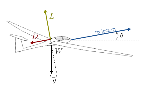
Lift, drag, and weight acting on a glider whose trajectory angle is positive above the horizontal — Figure 1:Forces on a glider with a positive trajectory angle.

On paper

Follow along the derivation of the mathematical model and keep those notes handy when you begin reconstructing the code for the numerical solution. This will help you not only create a base of understanding but create awareness to spot things like a pesky sign error.

In Figure 1, $L$ is lift, $W=mg$ is weight, $D$ is drag, and $\theta$ is the instantaneous trajectory angle. Resolving Newton’s second law parallel and perpendicular to the trajectory gives

\begin{aligned} m\frac{dv}{dt} &= -W\sin\theta-D,\\ mv\frac{d\theta}{dt} &= -W\cos\theta+L. \end{aligned}

(1)

On the direction normal to the trajectory, we used that the aircraft travels a small distance $ds=Rd\theta$ along the curved trajectory, at a speed $v=ds/dt=R \, d\theta/dt$ . This helps us write the centripetal acceleration $v^2/R$ as $v\, d\theta/dt$ .

Dividing Equation 1 by the weight and adopting primes for the time derivative gives

\begin{aligned} \frac{v'}{g} &= -\sin\theta-\frac{D}{W},\\ \frac{v}{g}\theta' &= -\cos\theta+\frac{L}{W}. \end{aligned}

(2)

From Lesson 1, the lift-to-weight ratio is written in terms of the trim speed, $L/W=v^2/v_t^2$ . Lift and drag share the same dynamic-pressure factor:

L=C_LS\frac{1}{2}\rho v^2, \qquad D=C_DS\frac{1}{2}\rho v^2.

(3)

It follows from Equation 3 that $D/L=C_D/C_L$ . Substituting these relations into Equation 2 produces the nonlinear velocity-and-angle model:

\begin{aligned} v' &= -g\sin\theta -\frac{C_D}{C_L}\frac{g}{v_t^2}v^2,\\ \theta' &= -\frac{g}{v}\cos\theta +\frac{g}{v_t^2}v. \end{aligned}

(4)

The factor $C_D/C_L$ is the inverse of the aerodynamic efficiency $L/D$ . It supplies damping: when the drag coefficient is zero, the damping term disappears. More aerodynamically efficient aircraft therefore have a more weakly damped phugoid mode.

The initial value problem¶

To draw the flight path, we also integrate the spatial coordinates. The horizontal position $x$ and upward-positive altitude $y$ satisfy

\begin{aligned} x'(t) &= v\cos\theta,\\ y'(t) &= v\sin\theta. \end{aligned}

(5)

Together, Equation 4 and Equation 5 form a system of four first-order differential equations. We need one initial value for every state variable:

v(0)=v_0,\qquad \theta(0)=\theta_0,\qquad x(0)=x_0,\qquad y(0)=y_0.

(6)

Solve with Forward Euler¶

In your notebook

Reconstruct the model, functions, time integration, plots, and convergence study in your own notebook. The worked code deliberately keeps euler_step() visible: compare it with the agent-driven refactoring you completed in Lesson 2, and identify which part represents the numerical method and which part represents the new physical model.

Forward Euler replaces a time derivative by a forward difference. For the speed,

v'(t_n)\approx\frac{v^{n+1}-v^n}{\Delta t},

(7)

where the superscript $n$ identifies the state at time $t_n$ . Using the form of Equation 7 for each of the differential equations and solving for the next state gives

\begin{aligned} v^{n+1} &= v^n+\Delta t\left( -g\sin\theta^n -\frac{C_D}{C_L}\frac{g}{v_t^2}(v^n)^2 \right),\\ \theta^{n+1} &= \theta^n+\Delta t\left( -\frac{g}{v^n}\cos\theta^n +\frac{g}{v_t^2}v^n \right),\\ x^{n+1} &= x^n+\Delta t\,v^n\cos\theta^n,\\ y^{n+1} &= y^n+\Delta t\,v^n\sin\theta^n. \end{aligned}

(8)

Note that Equation 8 evaluates the complete right-hand side from the current state before updating any state variable. In other words, after evaluating all four derivatives, we advance the complete state together.

As before, we collect the state and its derivatives into vectors:

u= \begin{bmatrix} v\\ \theta\\ x\\ y \end{bmatrix}, \qquad u'=f(u)= \begin{bmatrix} -g\sin\theta-\dfrac{C_D}{C_L}\dfrac{g}{v_t^2}v^2\\ -\dfrac{g}{v}\cos\theta+\dfrac{g}{v_t^2}v\\ v\cos\theta\\ v\sin\theta \end{bmatrix}.

(9)

In vector form, one Forward Euler step is simply

u^{n+1}=u^n+\Delta t\,f(u^n).

(10)

We will adopt the modular approach from Lesson 2 after the agent-driven refactoring, where we defined a Python function for the system dynamics and another for the time stepping. This is the key transition: rhs_full_phugoid() represents the model with drag and returns four derivatives, but euler_step() still implements Equation 10 without needing to know the length or meaning of the state vector. That is the power of array operations!

We begin by importing Python’s array and plotting libraries using the conventional aliases: np for NumPy and plt for Matplotlib.

import numpy as np
import matplotlib.pyplot as plt

Next, we need to choose representative model parameters and initial conditions. Angles in the state are measured in radians because np.sin() and np.cos() expect radians. The ratio $C_L/C_D=40$ represents a reasonably efficient sailplane, and $v_t=30\ \mathrm{m/s}$ is a representative trim speed. These are exploratory values rather than a model of a particular aircraft.

# Model parameters.
g = 9.81        # gravitational acceleration (m/s**2)
v_t = 30.0      # trim speed (m/s)
C_D = 1. / 40.  # drag coefficient
C_L = 1.0       # lift coefficient

# Initial conditions.
v_0 = v_t      # speed (m/s)
theta_0 = 0.0  # trajectory angle (rad)
x_0 = 0.0      # horizontal position (m)
y_0 = 1000.0   # altitude (m)

The function below translates Equation 9 directly into code. The name rhs_full_phugoid distinguishes this nonlinear four-state model from the linear two-state function in the previous lesson. We’re also providing a detailed description of the function parameters and return values in the docstring: the commented block under the function name. This block is shown to the user when appending a question mark (?) to the function name, or using the built-in help() functionality.

def rhs_full_phugoid(u, C_L, C_D, g, v_t):
    '''Return the derivatives for the nonlinear, damped phugoid model.

    Parameters
    ----------
    u : np.ndarray
        State vector [v, theta, x, y].
    C_L : float
        Lift coefficient.
    C_D : float
        Drag coefficient.
    g : float
        Gravitational acceleration.
    v_t : float
        Trim speed.

    Returns
    -------
    np.ndarray
        Derivative vector [dv/dt, dtheta/dt, dx/dt, dy/dt].
    '''
    v, theta, x, y = u
    return np.array([
        -g * np.sin(theta) - (C_D / C_L) * (g / v_t**2) * v**2,
        -(g / v) * np.cos(theta) + (g / v_t**2) * v,
        v * np.cos(theta),
        v * np.sin(theta),
    ])

Compare each returned array entry with the corresponding row of Equation 9. The position values $x$ and $y$ do not appear on the right-hand side, but keeping them in the state lets the same integration loop advance both the flight dynamics and the trajectory.

The Forward Euler function has the same vector update as in the previous lesson. This version uses *args so it can forward the larger model-parameter list without naming those parameters.

def euler_step(u, f, dt, *args):
    '''Return the next state using one Forward Euler step.

    Parameters
    ----------
    u : np.ndarray
        State at the current time.
    f : callable
        Function that returns the state derivatives.
    dt : float
        Time-step size.
    *args
        Additional positional arguments passed to f.

    Returns
    -------
    np.ndarray
        State after one Forward Euler step.
    '''
    return u + dt * f(u, *args)

Python refresher — forwarding arguments with *args

In a function definition, *args collects any additional positional arguments into a tuple. The asterisk * is an operator that tells Python to bundle all remaining arguments together, while args is just a naming convention. The expression f(u, *args) expands that tuple when calling f. For example,

euler_step(u, rhs_full_phugoid, dt, C_L, C_D, g, v_t)

makes args equal to (C_L, C_D, g, v_t) inside euler_step(), so its call to f is equivalent to rhs_full_phugoid(u, C_L, C_D, g, v_t). The Euler function remains independent of the particular model. (Read the Python documentation about Arbitrary Argument Lists for more details.)

Now choose the final time $T$ and step size $\Delta t$ . The variable num_steps counts updates, while the time grid contains num_steps + 1 points because it includes both endpoints. np.empty() allocates a two-dimensional state-history array with one row per time step and four columns ordered as $[v,\theta,x,y]$ . In the for-loop, the function euler_step() is called to get the solution at time step n+1.

T = 100.0  # length of the time interval (s)
dt = 0.1   # time-step size (s)
num_steps = int(round(T / dt))
t = np.linspace(0.0, T, num=num_steps + 1)

# Store [v, theta, x, y] at every time step.
u_history = np.empty((num_steps + 1, 4))
u_history[0] = np.array([v_0, theta_0, x_0, y_0])

for n in range(num_steps):
    u_history[n + 1] = euler_step(
        u_history[n], rhs_full_phugoid, dt, C_L, C_D, g, v_t
    )

Plot the trajectory¶

The state history contains everything we need to plot the trajectory of the glider. We extract the position coordinates using array indexing. A colon in the row position selects every time point, while columns 2 and 3 contain horizontal position and altitude, respectively.^[1]

x = u_history[:, 2]
y = u_history[:, 3]

# Set the font family and size to use for Matplotlib figures.
plt.rcParams['font.family'] = 'serif'
plt.rcParams['font.size'] = 12

fig, ax = plt.subplots(figsize=(8,3))

ax.set_title(f'Glider trajectory over {T:g} s')
ax.set_xlabel('Horizontal position, x (m)')
ax.set_ylabel('Altitude, y (m)')
ax.grid()
ax.plot(x, y, color='tab:red', linestyle='-', linewidth=2)
fig.tight_layout()

Grid convergence¶

In Lesson 2, when we studied the straight-line phugoid under a small perturbation, we looked at convergence by comparing the numerical solution with the exact solution. But we do not have an exact solution for this full nonlinear model. Instead, we compare solutions computed with different time-step sizes against the solution on a fine grid.

The finest-grid result is a numerical reference, not an exact solution. The resulting differences provide evidence of grid convergence only if the reference grid is sufficiently resolved and all compared grids represent the same initial-value problem over the same interval.

Compute a state history for each time-step size:

dt_values = [0.1, 0.05, 0.01, 0.005, 0.001]
u_histories = [] # an empty list for the solution on each grid

for dt_trial in dt_values:
    num_steps_trial = int(round(T / dt_trial))
    u_trial = np.empty((num_steps_trial + 1, 4))
    u_trial[0] = np.array([v_0, theta_0, x_0, y_0])

    for n in range(num_steps_trial):
        u_trial[n + 1] = euler_step(
            u_trial[n],
            rhs_full_phugoid,
            dt_trial,
            C_L,
            C_D,
            g,
            v_t,
        )

    u_histories.append(u_trial)

To compare arrays sampled on different grids, their time points must align. For nested grids, the refinement ratio $r=\Delta t_{\mathrm{coarse}}/\Delta t_{\mathrm{fine}}$ is an integer: every coarse-grid time is also a fine-grid time. A strided slice, which extracts elements from an array at regular intervals, can then select the fine-grid values that correspond to the coarse grid.

Python refresher — slicing with a stride

A one-dimensional NumPy slice has the form array[start:stop:stride]. Omitting start and stop selects the full array, while stride determines how many indices to advance each time. For example:

q = np.array([0, 10, 20, 30, 40, 50, 60])
q[::3]  # array([0, 30, 60])

In q_fine[::refinement_ratio] below, the slice begins at the shared initial time and keeps every $r$ th fine-grid value. A slice only selects array indices; it does not know what physical times those indices represent. That is why the nesting check must come before the slice.

The function below calculates refinement_ratio from the two time-step sizes. round() accommodates their floating-point representation, after which np.isclose() verifies that $\Delta t_{\mathrm{coarse}}\approx r\,\Delta t_{\mathrm{fine}}$ . If this relation fails, strided slicing cannot make a valid time-by-time comparison; interpolation would be needed, and we deliberately avoid introducing that additional approximation here. raise ValueError(... means: “This input is unacceptable; stop this function and report an error.”

After slicing, the shape check confirms that the endpoints and sample counts also align. Because every grid in this lesson begins at zero and ends at the same $T$ , the spacing and shape checks together establish that corresponding entries represent the same times. The generic names q_coarse and q_fine make clear that the function compares one sampled quantity; below, that quantity will be horizontal position.

def discrete_l1_difference(
    q_coarse, q_fine, dt_coarse, dt_fine
):
    '''Return a discrete L1 difference on two nested time grids.'''
    refinement_ratio = int(round(dt_coarse / dt_fine))

    if not np.isclose(
        dt_coarse, refinement_ratio * dt_fine
    ):
        raise ValueError('Time-step sizes do not define nested grids.')

    q_fine_on_coarse_grid = q_fine[::refinement_ratio]

    if q_fine_on_coarse_grid.shape != q_coarse.shape:
        raise ValueError('Grid endpoints or sample counts do not align.')

    return dt_coarse * np.sum(
        np.abs(q_coarse - q_fine_on_coarse_grid)
    )

Now we can use the function to compute the differences between the $x$ positions that were computed with each different value of the time step $\Delta t$ and the reference values on the finest grid. These differences will be used to analyze convergence below.

Python refresher — pairing sequences with zip()

The built-in Python function zip() pairs items that occupy the same position in two or more sequences. A for loop can unpack each pair directly into separate names:

letters = ['a', 'b', 'c']
numbers = [1, 2, 3]

for letter, number in zip(letters, numbers, strict=True):
    print(letter, number)

Without strict=True, zip() stops when the shortest input is exhausted, which can conceal a length mismatch. With strict=True, Python raises a ValueError instead.

dt_reference = dt_values[-1]
x_reference = u_histories[-1][:, 2]
difference_values = []

for dt_trial, u_trial in zip(
    dt_values[:-1], u_histories[:-1], strict=True
):
    x_trial = u_trial[:, 2]
    difference_values.append(
        discrete_l1_difference(
            x_trial,
            x_reference,
            dt_trial,
            dt_reference,
        )
    )

The assignments before the loop select the finest-grid data as the numerical reference: the index -1 means the final item, and column 2 of the state history contains horizontal position. The slices [:-1] then exclude that reference from both sequences, so we do not compare the finest solution with itself.

Each entry in u_histories was generated from the time-step size at the same position in dt_values. The call to zip(..., strict=True) pairs those corresponding entries and verifies that the two sliced sequences have equal lengths. The loop can therefore be read almost as prose: for each trial time step and its corresponding state history do something (compute the differences).

Inside the loop, x_trial = u_trial[:, 2] extracts the horizontal-position history, discrete_l1_difference() compares it with x_reference, using both time-step sizes to align the grids, and .append() stores the resulting difference in the same order as the coarser entries of dt_values.

We’re ready to make a plot of our analysis. Like in Lesson 2, we use a log-log plot to visualize a power-law relationship.

dt_array = np.array(dt_values[:-1])

fig, ax = plt.subplots(figsize=(5.0, 5.0))
ax.set_title(r'$L_1$ difference vs. time-step size')
ax.set_xlabel(r'$\Delta t$ (s)')
ax.set_ylabel(r'$L_1$ difference in $x$')
ax.grid()
ax.loglog(
    dt_array,
    difference_values,
    color='tab:blue',
    linestyle='--',
    marker='o',
)
ax.set_aspect('equal', adjustable='box')
fig.tight_layout()

As the time step decreases, the difference from the finest-grid reference also decreases. This is useful numerical evidence, but it does not yet prove convergence because the finest reference is not exact.

Observed order of convergence¶

Systematic grid-refinement studies and estimates of observed order are standard tools in numerical-solution verification Roache, 1998 Oberkampf & Roy, 2010. As you increasingly adopt agentic coding, having a strong foundation on these techniques will be ever more important.

Suppose three step sizes have a constant refinement ratio $r$ , with $f_1$ the finest-grid result and $f_3$ the coarsest. Let $D_{21}$ be a norm of the difference between the medium and fine results, and $D_{32}$ the corresponding difference between the coarse and medium results. The observed order of convergence is:

p= \frac{\log(D_{32}/D_{21})}{\log r}.

(11)

For a first-order method in its asymptotic range, we expect $D_{32}/D_{21}\approx r$ and therefore $p\approx1$ . We use three nested grids with $r=2$ .

Verification study with an agent¶

Verification studies are necessary for computational credibility, but they often require repetitive integrations, grid alignment, comparisons, and reporting. An agent can reduce that workload and make these frequently neglected activities more practical. It cannot decide which claim matters, whether the experiment actually tests that claim, or whether the evidence is sufficient. Those responsibilities remain yours.

With an agent

You already have all the ingredients:

The three-grid formula for $p$ .
The expectation $p\approx1$ for Forward Euler.
A function for comparing histories on nested grids.
Experience generating solutions with several time steps.
A working nonlinear model and Euler step.

Use an agent to add and run a bounded observed-order investigation in your notebook. In the previous lesson, the agent returned a proposal that you installed and tested. Here, after you complete the specification below, the agent may inspect your notebook, add new cells, execute them locally, and revise only its own additions. You will inspect the work, reproduce its arithmetic, and reach the final verdict.

On paper

Establish expectations before asking the agent to calculate anything. Let $f_1$ be the finest-grid solution, set $r=2$ and $\Delta t_1=0.001\ \mathrm{s}$ , and answer:

What are the medium and coarse time-step sizes $\Delta t_2$ and $\Delta t_3$ ?
Which pair of solutions defines $D_{21}$ , and which defines $D_{32}$ ?
Which difference should be larger for a converging calculation?
For first-order behavior, what approximate value do you expect for $D_{32}/D_{21}$ ?
Substitute that expected ratio into Equation 11. What value of $p$ do you predict?

Record your answers before delegation. They are independent expectations against which you will audit the agent’s experiment; do not revise them merely to match its output.

Complete the task specification¶

Create a Markdown cell in your notebook titled Agent observed-order task brief and complete the four headings below. The directions under each heading are requirements for your specification, not text to send unchanged. Your brief should be precise enough that another person could tell whether the requested experiment was carried out, without prescribing every line of code.

Goal and scope: State the numerical claim being investigated, identify horizontal position $x(t)$ as the quantity to compare, and name your notebook as the artifact in which the agent will add the investigation. Keep physical-model validation, other integrators, and the paper-airplane challenge in Lesson 4 out of scope.
Non-negotiables: Record your three calculated step sizes in fine-to-coarse order; the definitions of $D_{21}$ and $D_{32}$ ; the formula for $p$ ; and the existing model, Euler step, initial-value problem, final time, and comparison function that must remain unchanged. Require column 2 of the state history and nested-grid comparisons without interpolation.
Allowed actions: Grant only the access needed to inspect your notebook, add new cells after this section, execute the required local cells, and revise the new cells if they fail. Explicitly address changes to existing cells, other files, package installation, and network access.
Done when: Require the agent to expose the three step sizes and step counts, $D_{21}$ , $D_{32}$ , their ratio, the calculated $p$ , execution status, and a short record of its changes. The result $p\approx1$ is the hypothesis under investigation, not a completion condition: an unexpected result must be reported rather than tuned away.

Compare the completed brief with the minimum sufficient specification. Resolve any consequential ambiguity before granting edit or execution access.

Invoke the agent¶

Save your notebook so the attached artifact contains your independent expectations and completed task brief. Configure the permissions recorded in the brief, attach the saved notebook, and send this short request:

Prompt

Read the completed section titled “Agent observed-order task brief” in the attached notebook. Carry out the specified numerical investigation, including the permitted notebook edits and execution. Return the requested change record and numerical evidence. Do not broaden the investigation or make the final credibility judgment.

If you do not have access to an agent that can edit and execute a notebook, carry out the completed specification yourself and use the same audit and verdict below. The instructor can provide the reference result after you have recorded your own evidence.

Audit the implementation and evidence¶

Inspect the cells the agent added before accepting them. Do not judge the work from the final value of $p$ alone. Check that:

the grids are ordered fine, medium, and coarse, with the constant refinement ratio you specified;
every integration uses the same initial state, parameters, final time, rhs_full_phugoid(), and euler_step();
column 2, horizontal position, is compared on aligned grids using discrete_l1_difference();
$D_{21}$ is the medium--fine difference, $D_{32}$ is the coarse--medium difference, and their ratio appears in the correct order in Equation 11;
the response exposes the raw differences, ratio, and $p$ , rather than only asserting that verification passed; and
no previous cells or out-of-scope artifacts were changed.

Run the accepted cells yourself. Independently divide the reported $D_{32}$ by $D_{21}$ and use that ratio to recalculate $p$ . If either value disagrees with the agent’s report, locate the discrepancy rather than changing the expected theory or suppressing the result.

Your verdict

Write a short debrief that answers:

Did you accept, revise, or reject the agent’s work? Cite the inspected code and numerical evidence behind that decision.
Does the experiment support first-order behavior for horizontal position over this grid family? Report $D_{21}$ , $D_{32}$ , their ratio, and $p$ .
Why is this evidence stronger than visual agreement between trajectories?
State at least two things that could still be wrong or unverified even if $p$ is close to 1.
Leave a lightweight agent record naming the agent or persona, attached notebook, request, access granted, cells accepted or revised, and verification you performed.

Completion rubric¶

This is a Complete/Revise checkpoint. Your independent expectation, specification, audit, evidence, and judgment are what matters. Every row must meet the Complete description. In particular, obtaining $p\approx1$ does not compensate for an incorrect or unaudited experiment.

Criterion	Complete	Revise
Independent expectation	Correctly orders the grids and predicts $D_{32}/D_{21}\approx2$ and $p\approx1$ before delegation.	Expectations are absent, recorded after delegation, or use incorrect grid or difference ordering.
Specification	Defines the claim, quantity, grids, difference mapping, formula, task boundary, and required evidence.	Leaves consequential numerical choices implicit or merely asks the agent to “check convergence.”
Access and scope	Grants bounded notebook inspection, new-cell editing, and local execution while protecting existing work.	Gives unbounded access or permits changes to the model, Euler step, problem data, or prior results.
Code audit	Checks state indexing, common problem data, grid nesting, difference ordering, and the observed-order formula.	Judges primarily from the final value or accepts the response without inspecting its implementation.
Reproducible evidence	Records all step sizes and counts, both raw differences, their ratio, $p$ , and the execution result.	Reports only that $p$ is close to one or repeats an unsupported assurance that checks passed.
Verdict and limitations	Connects the evidence to a bounded claim and identifies what remains unverified.	Treats observed order as proof that the model and complete calculation are correct.
Provenance	Records the agent, artifact, request, permitted actions, accepted changes, and learner-run verification.	Material agent work or subsequent human corrections are not recorded.

What’s next?¶

This lesson marched the full, damped phugoid model forward with Euler’s method and used grid refinement to assess convergence without an exact solution. In Lesson 4, a paper-airplane challenge turns method choice into an exercise in engineering judgment. You will introduce explicit midpoint RK2, build and verify a touchdown-range calculation, and use refinement evidence to decide when a predicted range is accurate enough. You will then compare Euler and RK2 by computational cost and supervise agent-authored search code while retaining responsibility for execution and the final verdict.

Footnotes¶

For a quick review of Python indexing using simple strings, see this video by Prof. Barba.
↩

References¶

Roache, P. J. (1998). Verification and Validation in Computational Science and Engineering. Hermosa Publishers.
Oberkampf, W. L., & Roy, C. J. (2010). Verification and Validation in Scientific Computing. Cambridge University Press.