Phugoid Motion - Practical Numerical Methods

In the first module of “Practical Numerical Methods” we study problems modeled by ordinary differential equations.

Our motivating problem is the phugoid model of glider flight. In this first lesson, we discuss some background, explain the physics, and work out the mathematical model.

We first consider the idealized model with no drag, resulting in a simple harmonic motion. We can plot some interesting trajectories of a glider under phugoid oscillations. In the next lesson, you’ll learn to numerically integrate the differential equation using Euler’s method.

The term phugoid in aeronautics refers to a motion pattern where an aircraft oscillates up and down —nose-up and climb, then nose-down and descend— around an equilibrium trajectory. The aircraft oscillates in altitude, speed and pitch, with only small (neglected) variations in the angle of attack, as it repeatedly exchanges kinetic and potential energy Sinha & Ananthkrishnan, 2013, chap. 5.

A low-amplitude phugoid motion can be just a nuisance, as the aircraft does not exceed the stall angle of attack and nothing bad happens. But the mode can also be unstable leading to a stall or even a loop.

Look at this video of a simulator showing a Cessna single-engine airplane in phugoid motion:

from IPython.display import YouTubeVideo
YouTubeVideo('ysdU4mnRYdM')

That doesn’t look too good! What’s happening?

It can get a lot worse when an aircraft enters one of these modes that is unstable. A famous example is that of NASA’s Helios Solar Powered Aircraft prototype, which broke up in mid air due to extreme phugoid oscillations.

Helios was a proof-of-concept solar electric-powered flying wing that broke the world altitude record for a non-rocket-powered aircraft in August 2001. But in June 26, 2003, it broke something else. The aircraft entered phugoid motion after encountering turbulence near the Hawaiian Island of Kauai. The high speed reached in the oscillations exceeded the design limits, and it ended up wrecked in the Pacific Ocean. Luckily, the Helios was remotely operated, and nobody got hurt.

The physics of phugoids¶

In a phugoid oscillation the aircraft pitches up and down, as it decelerates and accelerates. The trajectory might look like a sinusoid, as shown in Figure 1. The assumption is that the forward velocity of the aircraft, $v$ , varies in such a way that the angle of attack remains (nearly) constant, which means that we can assume a constant lift coefficient.

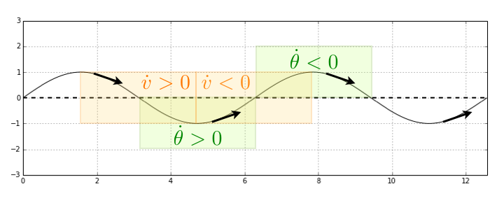
A sinusoidal trajectory showing an aircraft oscillating above and below a central flight path — Figure 1:Trajectory of an aircraft in phugoid motion.

In the descending portion of the trajectory, the aircraft’s velocity increases as it proceeds from a peak to the minimum height—gaining kinetic energy at the expense of potential energy. The contrary happens in the upward segment, as its velocity decreases there.

We measure the pitch angle (between the aircraft’s longitudinal axis and the horizontal) as positive when the aircraft’s nose is pointing up. In the portion of the trajectory below the center-line, where it curves upwards, the pitch angle $\theta$ is increasing: $\dot{\theta}>0$ . And where the trajectory curves down, the pitch angle is decreasing: $\dot{\theta}<0$ , as shown in Figure 1.

Let’s review the forces affecting an aircraft in a downward glide. In Figure 2, we show the flight path, the forces on the glider (no thrust), and the glide angle or flight path angle, $\gamma$ , between the flight path and the horizontal.

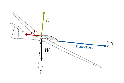
Lift, drag, and weight acting on a glider along a descending flight path — Figure 2:Forces on a glider.

The force of lift, $L$ —created by the airflow around the wings— is perpendicular to the trajectory, and the force of drag, $D$ , is parallel to the trajectory. Both forces are expressed in terms of coefficients of lift and drag, $C_L$ and $C_D$ , respectively, that depend on the wing design and angle of attack: the angle between the wing chord and the flight path.

If you are not familiar with airplane aerodynamics, you might be getting confused with some terms here ... and all those angles! But be patient and look things up, if you need to. We’re giving you a quick summary here.

Lift and drag are proportional to a surface area, $S$ , and to the dynamic pressure: $1/2 \rho v^2$ , where $\rho$ is the density of air, and $v$ the forward velocity of the aircraft. The equations for lift and drag are:

L = C_L S \times \frac{1}{2} \rho v^2

(1)

D = C_D S \times \frac{1}{2} \rho v^2

(2)

When the glider is in equilibrium, the forces balance each other. We can equate the forces in the directions perpendicular and parallel to the trajectory, as follows:

L = W \cos \gamma \quad \text{and} \quad D = W \sin \gamma

(3)

where $W$ represents the weight of the glider.

In the figure, we’ve drawn the angle $\gamma$ as the glide angle, formed between the direction of motion and the horizontal. We are not bothered with the sign of the angle, because we draw a free-body diagram and take the direction of the forces into account in writing our balance equations. But later on, we will need to be careful with the sign of the angles. It can cause you a real headache to keep this straight, so be patient!

Below, we will develop the mathematical model step-by-step. But before, a short glimpse of the history.

Lanchester’s Aerodonetics¶

“Phugoid theory” was first described by the British engineer Frederick W. Lanchester in Aerodonetics Lanchester, 1908. The book is now in the public domain, so you can read or download it from the Internet Archive.

Lanchester defines phugoid theory as the study of longitudinal stability of a flying machine (aerodone). He first considered the simplification where drag and moment of inertia are neglected. Then he included these effects, obtaining an equation of stability. In addition to describing many experiments by himself and others, Lanchester also reports on “numerical work ... done by the aid of an ordinary 25-cm slide rule” Lanchester, 1908. Go figure!

Ideal case of zero drag¶

In this section, we follow the derivation given by Milne-Thomson (1966, sec. 18.5), which we find a little bit easier than that of the original in “Aerodonetics.”

An aircraft flying in steady, straight horizontal flight has a lift equal to its weight. The velocity in this condition is sometimes called trim velocity (“trim” is what pilots do to set the controls to just stay in a steady flight). Let’s use $v_t$ for the trim velocity, and from $L=W$ deduce that:

W = C_L S \times\frac{1}{2} \rho v_t^2

(4)

The weight $W$ is constant for the aircraft, but the lift at any other flight condition depends on the flight speed, $v$ . We can use the expression for the weight in terms of $v_t$ to obtain the ratio $L/W$ at any other flight velocity, as follows:

\frac{L}{W}= \frac{v^2}{v_t^2}

(5)

Imagine that the aircraft experienced a little upset, a wind gust, and it finds itself off the “trim” level, in a curved path with an instantaneous angle $\theta$ . In Figure 3, we exaggerate the curved trajectory of flight to help you visualize what we’ll do next. The angle $\theta$ (using the same name as Milne-Thompson) is between the trajectory and the horizontal, positive up.

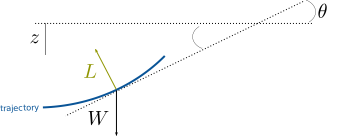
Curved upward trajectory of an aircraft with lift and weight vectors — Figure 3:Curved trajectory of an aircraft climbing with no drag.

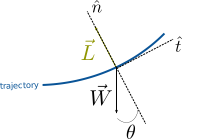
Free-body diagram showing lift, weight, and normal and tangential directions — Figure 4:Free-body diagram of the aircraft trajectory.

From Figure 4, we can see that

\vec{L} + \vec{W} = m\vec{a} = \frac{mv^2}{R}\hat{n} + m \frac{dv}{dt}\hat{t}

(6)

where $\frac{v^2}{R}$ is the centripetal acceleration and $R$ is the radius of curvature of the trajectory. If we decompose the lift and weight into their normal and tangential components we get

L\hat{n} + W_n\hat{n} + W_t\hat{t} = \frac{mv^2}{R}\hat{n} + m \frac{dv}{dt}\hat{t}

(7)

The component of the weight in the normal direction ( $W_n$ ) is

W_n = -W \cos \theta

(8)

If we then consider that all of the components in $\hat{n}$ must balance out, we arrive at

L - W \cos \theta = \frac{mv^2}{R}

(9)

We can rewrite this as

L- W \cos \theta = \frac{W}{g} \frac{v^2}{R}

(10)

where $g$ is the acceleration due to gravity. Rearrange this by dividing the equation by the weight, and use the expression we found for $L/W$ , above. The following equation results:

\frac{v^2}{v_t^2}-\cos \theta = \frac{v^2}{g R}

(11)

Recall that we simplified the problem assuming that there is no friction, which means that the total energy is constant (the lift does no work). If $z$ represents the depth below a reference horizontal line, the energy per unit mass is (kinetic plus potential energy):

\frac{1}{2}v^2-g z = \text{constant}

(12)

To get rid of that pesky constant, we can choose the reference horizontal line at the level that makes the constant energy equal to zero, so $v^2 = 2 g z$ . That helps us re-write the phugoid equation in terms of $z$ as follows:

\frac{z}{z_t}-\cos \theta = \frac{2z}{R}

(13)

Let $ds$ represent a small arc-length of the trajectory. We can write

\frac{1}{R} = \frac{d\theta}{ds} \quad \text{and}\quad \sin\theta = -\frac{dz}{ds}

(14)

Employing the chain rule of calculus,

\frac{1}{R} = \frac{d\theta}{ds} = \frac{dz}{ds}\frac{d\theta}{dz} = -\sin \theta\frac{d\theta}{dz}

(15)

Multiply the phugoid equation by $\frac{1}{2\sqrt{z}}$ to get:

\frac{\sqrt{z}}{2z_t} - \frac{\cos\theta}{2\sqrt{z}} = \frac{\sqrt{z}}{R}

(16)

Substituting for $1/R$ on the right hand side and bringing the cosine term over to the right, we get:

\frac{\sqrt{z}}{2z_t} = \frac{\cos \theta}{2 \sqrt{z}} - \sqrt{z} \sin \theta \frac{d\theta}{dz}

(17)

The right-hand-side is an exact derivative! We can rewrite it as:

\frac{d}{dz} \left(\sqrt{z}\cos\theta \right) = \frac{\sqrt{z}}{2z_t}

(18)

Integrating this equation, we add an arbitrary constant, chosen as $C\sqrt{z_t}$ which (after dividing through by $\sqrt{z}$ ) gives:

\cos \theta = \frac{1}{3}\frac{z}{z_t} + C\sqrt{\frac{z_t}{z}}

(19)

Taking the derivative of both sides of Equation 19 and applying the relation in Equation 15 yields:

\frac{z_t}{R} = \frac{1}{3} - \frac{C}{2}\sqrt{\frac{z_t^3}{z^3}}

(20)

On paper

Before using code, reproduce the pivotal part of the derivation by hand:

Starting from Equation 19, differentiate with respect to $z$ and use Equation 15 to obtain Equation 20.
Check that $C$ and $z_t/R$ are dimensionless.
For $z_t=64$ , $z_0=16$ , and $\theta_0=0$ , calculate $C$ and predict the sign of the initial radius of curvature $R$ .
Sketch which way the trajectory should initially bend.

Keep this work beside you. Its values and predictions are independent evidence for checking the computation that follows. See Before computing for the general role of these checks.

Phugoid Curves¶

Equation 19 is nonlinear, so we are hard-pressed to write a clean expression for the complete path $z(x)$ . Lanchester said that he was unable to “reduce this expression to a form suitable for co-ordinate plotting.” Instead, he devised what he called the “trammel” method. His explanation begins on page 48 of Aerodonetics Lanchester, 1908, p. 48.

Lanchester used Equation 19 to calculate the integration constant $C$ and Equation 20 to calculate the local radius of curvature $R$ , then constructed the trajectory as a succession of small circular arcs—by hand.

We will now reproduce that process computationally. We will use this exercise explicitly as a Python refresher while we explore the simplest, zero-drag phugoid model.

If your Python is rusty, take time with the reminders and reconstruct one small step at a time in your own notebook. If you are already an experienced programmer, focus on how the mathematics becomes a small set of explicit functions, how computation is separated from plotting, and where we check the model’s domain instead of hiding numerical warnings.

The computational idea is simple: start from an initial point and angle, take a short step of arc length $ds$ , calculate the local circle from $R$ , rotate the point around that circle, and repeat.

Computational interlude: Python refresher¶

In your notebook

Create a new notebook for your work; do not execute code in this lesson notebook. Keep the lesson open as a reference and reconstruct the trammel calculation there.

Before running your first calculation, record the value of $C$ , the sign of $R$ , and the initial direction you predicted on paper. Type the equations, geometric update, loop, and model checks yourself. You may copy small mechanical elements such as imports or plot labels when transcription would add no understanding.

As you proceed, compare each computed result with your prediction and explain any disagreement before continuing. Consult Reconstruct a lesson for the general workflow.

We need two widely used scientific-Python packages: NumPy for numerical functions and arrays, and Matplotlib for plotting.

import numpy as np
import matplotlib.pyplot as plt

Translate the equations into functions¶

First, solve Equation 19 for $C$ at a known point $(z,\theta)$ :

C = \left(\cos\theta - \frac{z}{3z_t}\right)\sqrt{\frac{z}{z_t}}.

(21)

Equation 20 gives the corresponding signed radius of curvature:

R = \frac{z_t}{\frac{1}{3} - \frac{C}{2}\left(\frac{z_t}{z}\right)^{3/2}}.

(22)

The next cell translates those equations almost literally.

Both $z$ and $z_t$ represent positive depths. We check that assumption explicitly. A zero denominator in the second equation means a straight path with infinite radius, represented by np.inf.

def integration_constant(z, z_t, theta):
    '''Return the integration constant C; theta is in radians.'''
    if z <= 0.0 or z_t <= 0.0:
        raise ValueError("z and z_t must be positive.")
    return (np.cos(theta) - z / (3.0 * z_t)) * np.sqrt(z / z_t)


def radius_of_curvature(z, z_t, C):
    '''Return the signed local radius of curvature.'''
    if z <= 0.0 or z_t <= 0.0:
        raise ValueError("z and z_t must be positive.")
    denominator = 1.0 / 3.0 - C / 2.0 * (z_t / z)**1.5
    if np.isclose(denominator, 0.0):
        return np.inf
    return z_t / denominator

Let’s evaluate the two functions at one initial condition. Angles may be convenient to specify in degrees, but NumPy’s trigonometric functions expect radians, so we convert at the boundary between user input and computation.

A signed $R$ records which side of the trajectory contains the center of curvature; its magnitude is the geometric radius.

z_t = 64.0
z_0 = 16.0
theta_0_degrees = 0.0
theta_0 = np.deg2rad(theta_0_degrees)

C = integration_constant(z_0, z_t, theta_0)
R_0 = radius_of_curvature(z_0, z_t, C)

print(f"C = {C:.3f}")
print(f"Initial signed radius R = {R_0:.3f}")
assert 0.0 < C < 2.0 / 3.0

Rotate one point around a local circle¶

To follow one short circular arc, we rotate the current point $(x,z)$ about the center of curvature. The formula below is a standard two-dimensional rotation written for the sign convention used in our diagram.

def rotate_point(x, z, center, angle):
    '''Rotate the point (x, z) about center by angle radians.'''
    x_center, z_center = center
    dx, dz = x - x_center, z - z_center

    x_new = x_center + dx * np.cos(angle) + dz * np.sin(angle)
    z_new = z_center - dx * np.sin(angle) + dz * np.cos(angle)
    return x_new, z_new

March along the trajectory¶

We now have the pieces needed to imitate Lanchester’s trammel. The function below repeatedly calculates $R$ , locates the center of curvature, and rotates the current point through the small angle $d\theta=ds/R$ .

Notice two model-aware branches. An infinite radius produces a straight segment. Also, the ideal formula assumes positive depth $z$ ; rather than suppressing warnings after leaving that domain, we stop the trace before $z$ becomes non-positive.

Read this code carefully and convince yourself that it matches our model.

def trace_phugoid(z_t, z_0, theta_0, n_steps=1000, ds=1.0):
    '''Trace a zero-drag phugoid; theta_0 is supplied in degrees.'''
    if n_steps < 2:
        raise ValueError("n_steps must be at least 2.")

    theta = np.deg2rad(theta_0)
    C = integration_constant(z_0, z_t, theta)
    if C > 2.0 / 3.0 + 1e-12:
        raise ValueError("These initial conditions give C > 2/3.")

    x_values = [0.0]
    z_values = [z_0]

    for _ in range(n_steps - 1):
        x_current, z_current = x_values[-1], z_values[-1]
        R = radius_of_curvature(z_current, z_t, C)

        if np.isinf(R):
            dtheta = 0.0
            x_new = x_current + ds * np.cos(theta)
            z_new = z_current - ds * np.sin(theta)
        else:
            normal = np.array([-np.sin(theta), -np.cos(theta)])
            center = np.array([x_current, z_current]) + R * normal
            dtheta = ds / R
            x_new, z_new = rotate_point(
                x_current, z_current, center, dtheta
            )

        if z_new <= 0.0:
            break

        x_values.append(x_new)
        z_values.append(z_new)
        theta += dtheta

    return np.asarray(x_values), np.asarray(z_values), C

Keep plotting separate from computation¶

The trajectory function returns numerical data without deciding how it must be displayed. A second, smaller function handles the plot. This separation lets us inspect, test, or reuse the coordinates without producing a figure every time.

Our coordinate $z$ is depth measured positive downward, so the plot uses $-z$ to show upward displacement in the familiar direction.

def plot_flight_path(x, z, C):
    '''Plot a previously computed phugoid trajectory.'''
    fig, ax = plt.subplots(figsize=(9.0, 4.0))
    
    ax.plot(x, -z, linewidth=2.0)
    ax.set_title(f"Flight path for C = {C:.3f}")
    ax.set_xlabel(r"$x$")
    ax.set_ylabel(r"$-z$")
    ax.grid()
    ax.set_aspect("equal", adjustable="box")
    return fig, ax

Explore the family of phugoid curves¶

Look again at Equation 19. The value of $C$ organizes the possible paths:

$C>2/3$ gives no physical solution because it would require $\cos\theta>1$ .
$C=2/3$ gives the horizontal straight path: $\theta=0$ and $R=\infty$ .
$0<C<2/3$ gives trochoidal-like paths.
$C<0$ can give paths containing loops.
$C=0$ makes $R=3z_t$ , a constant.

First choose conditions that give $0<C<2/3$ . Before running the cell, predict the sign of the initial curvature and the general shape of the path.

x, z, C = trace_phugoid(z_t=64.0, z_0=16.0, theta_0=0.0)
fig, ax = plot_flight_path(x, z, C)

The calculated value is $C\approx0.458$ , between 0 and $2/3$ , and the path is trochoidal as predicted.

Now keep the two depths fixed but reverse the initial direction to $180^\circ$ . What sign do you predict for $C$ ? What new feature should appear in the path?

x, z, C = trace_phugoid(z_t=64.0, z_0=16.0, theta_0=180.0)
fig, ax = plot_flight_path(x, z, C)

The negative value of $C$ produces loops. Experiment by changing one input at a time and predicting the result before you run the cell again.

For a more experienced Python programmer, this is also a useful design question: which conditions belong in input validation, which are mathematical limiting cases, and which should eventually become automated tests?

For $C=0$ , Equation 20 reduces to

R=3z_t.

(23)

The radius is constant. Setting $z_0=3z_t$ and $\theta_0=0$ forces $C=0$ . Our ideal model is defined only for $z>0$ , so the tracer follows the circular arc until just before it reaches the reference level.

x, z, C = trace_phugoid(z_t=16.0, z_0=48.0, theta_0=0.0)
fig, ax = plot_flight_path(x, z, C)

The result is a quarter-circle arc with radius $48=3z_t$ . We can obtain an almost semicircular path from another configuration where $C$ is close to zero:

x, z, C = trace_phugoid(z_t=64.0, z_0=16.0, theta_0=-90.0)
fig, ax = plot_flight_path(x, z, C)

With an agent

Use an agent to help evaluate your reconstructed trace_phugoid() function—not to replace it. Before invoking the agent, specify that it should leave the implementation unchanged and propose independent validation checks using only NumPy. For every check, require the agent to name the mathematical property being tested and a plausible defect the check could expose. If this is your first agent task, review Define the task by specification.

Ask for checks covering at least these cases:

Horizontal limit: $z_0=z_t$ and $\theta_0=0$ give $C=2/3$ , constant $z$ , and a straight path.
Circular limit: $z_0=3z_t$ and $\theta_0=0$ give $C=0$ and points satisfying $x^2+z^2=(3z_t)^2$ .
Model domain: non-positive depths, too few steps, and initial conditions giving $C>2/3$ should fail clearly.

Review the proposed checks before running them. Then reverse the sign of dtheta in a temporary copy of your function and see whether the checks detect motion around the circle in the wrong direction. If they do not, improve the suite with an orientation check based on your paper sketch. This combines comparison with known behavior and deliberate defect injection. Record which agent suggestions you accepted, rejected, or corrected.

We have reproduced trajectories that Lanchester painstakingly constructed by hand with his trammel. Along the way, we refreshed imports, function definitions, assignments, tuples, lists, arrays, loops, conditionals, exceptions, formatted strings, and object-oriented plotting.

More importantly, every code element corresponds to a modeling choice: the sign convention, the domain $z>0$ , the local radius, and the discrete arc-length step. Python is the medium, but the computational argument comes from the model.

Figure 5 reproduces the phugoid curves from von Kármán’s Aerodynamics. He never says how he drew them, but we’re guessing by hand, too. We did pretty well!

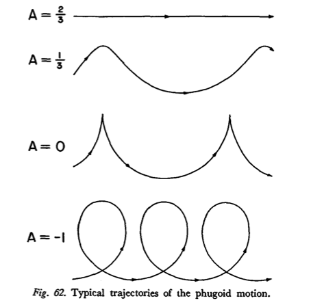
A family of looping and cusped phugoid trajectories — Figure 5:Phugoid curves in von Kármán’s *Aerodynamics* Kármán, 1954, pp. 149–151.

Your verdict

Conclude your notebook with a short engineering verdict:

Which check provides the strongest evidence that your tracer implements the intended model, and why?
Which plausible defect could have escaped the agent’s original checks?
What have you verified about the computation, and what remains unverified?

State whether you accept the implementation, accept it with limitations, or require revision. Support that decision with evidence rather than the fact that the code ran or the tests passed. Use the short evidence record and leave a lightweight agent record.

This trammel algorithm marched geometrically along the trajectory in increments of arc length $ds$ . In the next lesson, we will derive the differential equation for a small perturbation of the horizontal phugoid and march a dynamical state forward in time using Euler’s method. The same computational patterns—state, steps, loops, updates, and inspection—will reappear in a new numerical setting.